Testing whiteness of residuals, Choosing Q and R, Outliers, faults and modelling errors, Time-varying systems, Coloured noise, Numerical issues, Nonlinear systems (12.03 - 12.10)

What does testing the whiteness of residuals mean?

Testing whiteness assesses whether the residuals (or normalized innovations) are uncorrelated over time (i.e., white noise). This ensures that the residuals are independent at different time steps, which is a critical assumption for a correctly functioning Kalman filter.

For normalized residuals \tilde{\nu}_k, the condition is:

E[\tilde{\nu}_k \tilde{\nu}_{k+\ell}^\top] = I \delta_\ell,

where:

- I is the identity matrix,

- \delta_\ell is the Kronecker delta, meaning the residuals are uncorrelated except at zero lag (\ell = 0).

How is the autocorrelation of residuals calculated?

The estimated autocorrelation of the i-th element (only one element of v) of the residuals is:

\hat{R}_i(\ell) = \frac{1}{K - \ell} \sum_{k=1}^K [\tilde{\nu}_k]_i [\tilde{\nu}_{k+\ell}]_i,

where:

- K is the number of data points,

- \ell is the lag.

For \ell \neq 0 (we vary l), the statistic:

\sqrt{K} \frac{\hat{R}_i(\ell)}{\hat{R}_i(0)} \sim N(0, 1),

is a random variable that follows a standard normal distribution.

We want to see if this estimated autocorrelation (taken from the Kalman filter) matches the hypothetical requirements described in the previous flashcard. To be reasonably close to the ideal condition, the above result must be normally distributed with unit variance.

How can whiteness be tested with 95% confidence?

To test if residuals are white with 95% confidence, check that:

\frac{\hat{R}_i(\ell)}{\hat{R}_i(0)}

lies within:

\pm \frac{1.96}{\sqrt{K}},

for \ell = 1, 2, \dots.

This is done by plotting \hat{R}_i(\ell)/\hat{R}_i(0) against \ell and verifying if the values stay within the bounds.

The red lines represent the +- 1.96 restriction. If you were to take all these autocorrelation values over time and put them into a graph of common values, it would form a normal distribution curve.

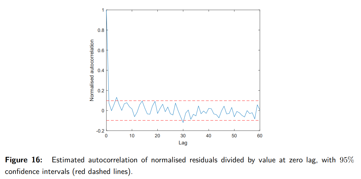
What does Example 28 illustrate about whiteness testing?

In Example 28, the autocorrelation of normalized innovations from the Kalman filter estimates (Figure 16) is plotted, scaled by the autocorrelation at zero lag. Most data points lie within the 95% confidence interval (red dashed lines). This confirms that the innovations are white, validating the Kalman filter's assumptions.

What is the challenge in selecting Q and R in the Kalman filter?

Selecting Q (process noise covariance) and R (measurement noise covariance) is challenging because their true values are often unknown. The process involves:

1. Running the Kalman filter with initial guesses for Q and R.

2. Checking if the normalized residuals \tilde{\nu}_k are both normally distributed and white.

3. Adjusting Q and R based on the test results.

For scalar systems:

- A low Q/R ratio results in non-white normalized residuals (shown in autocorrelation plots).

- Once a suitable Q/R ratio is found, Q and R can be scaled to satisfy normality and \chi^2 tests.

How are Q and R chosen for multivariate systems?

For systems with multiple measurements or noise sources, Q and R are matrices, making the selection process more complex. Even so, examining the normalized residuals remains a valuable tool for tuning these matrices.

What are outliers in measurement data, and how are they handled in the Kalman filter?

Outliers are large deviations in the measurement signal caused by sensor errors. These outliers disrupt the assumption of Gaussian noise. To handle them:

1. Monitor the normalized innovations \tilde{\nu}_k.

2. If |\tilde{\nu}_k| > 2.8, the corresponding measurement is identified as an outlier with 99.5% certainty (not Gaussian with unit variance).

3. For such measurements, the measurement update step in the Kalman filter is skipped to avoid corrupting the state estimate.

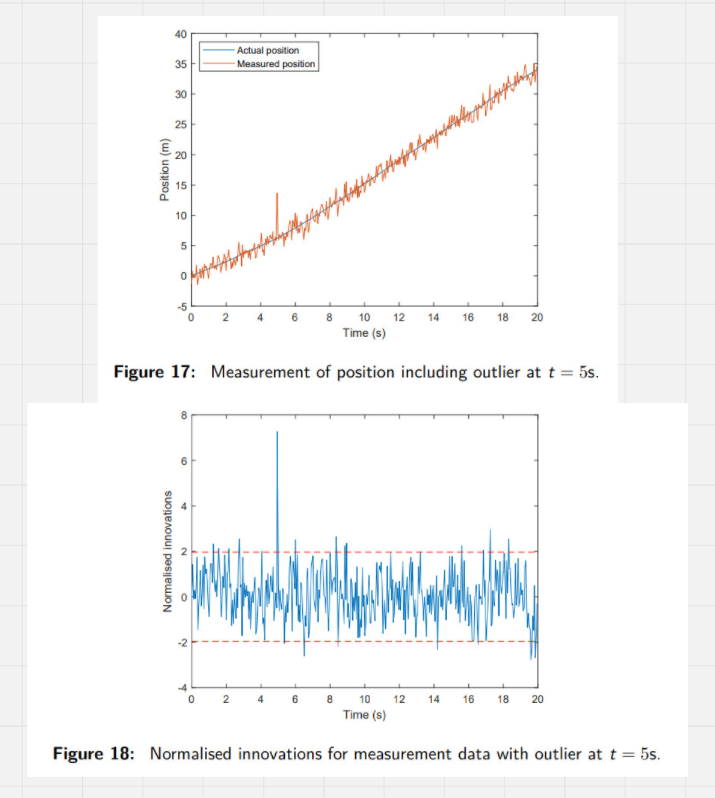
What does Example 29 demonstrate about outliers?

Example 29 illustrates noisy position measurements with an outlier at t = 5s:

- Figure 17: Shows the actual position, measured position, and the deviation caused by the outlier.

- Figure 18: The normalized innovations corresponding to the outlier exceed the 95% confidence bounds, enabling its detection.

How can normalized innovations be used to detect faults or modeling errors?

Monitoring normalized innovations helps detect changes in the system, such as:

- Sensor faults: Increase the variance of the measurement noise, leading to larger normalized innovations.

- Actuator faults: Change the system's dynamics, resulting in correlations in the residuals.

- Modeling errors: Caused by unmodeled dynamics or incorrect state-space representations, also leading to correlations in the residuals.

Self-validating sensors use Kalman filters to monitor normalized innovations and detect such faults.

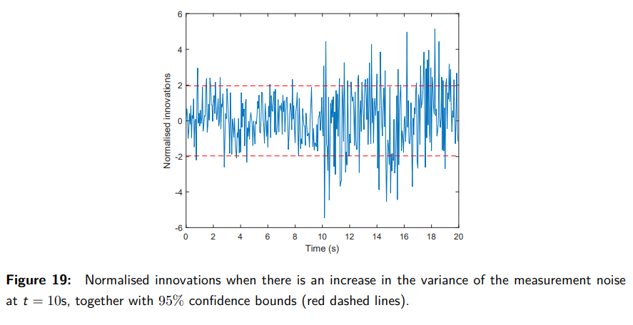
What does Example 30 illustrate about detecting changes in the system?

Example 30 shows the normalized innovations when the measurement noise variance increases from R = 1 to R = 2 at t = 10\text{s}:

- The magnitude of the normalized innovations increases significantly.

- This change is visible in Figure 19, along with the 95% confidence bounds (red dashed lines), demonstrating how the Kalman filter can detect such changes.

How does the Kalman filter handle time-varying systems?

For time-varying systems, the state-space model allows matrices to change over time:

x_{k+1} = A_d^k x_k + B_d^k u_k + G_d^k w_r^k,

y_k = C_k x_k + v_k,

with noise covariance matrices:

- Process noise:

E[w_r^k (w_r^k)^\top] = Q_r^k \delta_\ell,

- Measurement noise:

E[v_k v_k^\top] = R_k \delta_\ell,

- Cross-correlation:

E[w_r^k v_k^\top] = 0.

The noise sequences remain white, but the covariance matrices Q_r^k and R_k can vary with time.

What is the significance of time-varying models in the Kalman filter?

Time-varying models are important because:

1. They can describe systems with changing dynamics over time.

2. They accommodate cases where the sampling interval is not constant in discrete-time systems.

3. The derivations for both continuous-time and discrete-time Kalman filters remain valid for such models.

What is the Kalman filter for time-varying models?

For time-varying models, the Kalman filter equations are:

1. Prediction Step:

- State prediction:

\hat{x}_{k+1|k} = A_d^k \hat{x}_{k|k} + B_d^k u_k.

- Covariance prediction:

P_{k+1|k} = A_d^k P_{k|k} (A_d^k)^\top + G_d^k Q_r^k (G_d^k)^\top.

2. Measurement Update Step:

- Kalman Gain:

L_{k+1} = P_{k+1|k} (C_{k+1})^\top \left(C_{k+1} P_{k+1|k} (C_{k+1})^\top + R_{k+1}\right)^{-1}.

- State update:

\hat{x}_{k+1|k+1} = \hat{x}_{k+1|k} + L_{k+1} \left(y_{k+1} - C_{k+1} \hat{x}_{k+1|k}\right).

- Covariance update:

P_{k+1|k+1} = (I - L_{k+1} C_{k+1}) P_{k+1|k} (I - L_{k+1} C_{k+1})^\top + L_{k+1} R_{k+1} (L_{k+1})^\top.

Note: For time-varying systems, P_{k+1|k+1} does not converge to a steady-state value, and no algebraic Riccati equation exists.

What is colored noise, and how is it modeled?

Colored noise refers to noise with time correlation, unlike white noise, which is uncorrelated.

1. Process Noise:

Modeled as:

w_c^k = g_0 \frac{1}{z + f_1} n_k,

where n_k is a white noise process with covariance matrix:

E[n_k n_k^\top] = Q_n.

2. State-Space Representation for Colored Noise:

w_c^{k+1} = -f_1 w_c^k + g_0 n_k.

3. Augmented State-Space Model:

The process noise is incorporated into the system state:

\begin{bmatrix} x_{k+1} \\ w_c^{k+1} \end{bmatrix} = \begin{bmatrix} A & G \\ 0 & -f_1 \end{bmatrix} \begin{bmatrix} x_k \\ w_c^k \end{bmatrix} + \begin{bmatrix} B \\ 0 \end{bmatrix} u_k + \begin{bmatrix} 0 \\ g_0 \end{bmatrix} n_k.

The Kalman filter is applied to the augmented model.

How can colored measurement noise be handled?

Colored measurement noise is modeled similarly by augmenting the measurement noise into the state-space model. However, this violates the requirement that the covariance matrix R be positive definite, as R \succ 0.

What is the impact of colored noise on the Kalman filter?

- Increased State Dimension: Incorporating colored noise into the model increases the dimensionality of the state vector.

- Filter Design: The augmented state-space model is necessary to accurately account for noise correlations.

What are the numerical issues in Kalman filtering?

Numerical issues in Kalman filtering occur when the covariance matrix of estimation errors, P_{k|k}, becomes unstable. This instability arises due to numerical round-off errors during recursive computations on a computer. These errors can lead to:

1. Loss of Symmetry: P_{k|k} might no longer remain symmetric, which violates the assumptions of the Kalman filter.

2. Loss of Positive Definiteness: P_{k|k} may fail to remain positive definite, which is critical for correctly modeling uncertainty in state estimates.

If P_{k|k} becomes unstable, the Kalman filter's estimates can degrade or fail entirely.

How can numerical issues in Kalman filtering be avoided?

Numerical issues can be avoided by representing the covariance matrix P_{k|k} in terms of its matrix square root:

P_{k|k} = P_{k|k}^{1/2} \left(P_{k|k}^{1/2}\right)^\top,

where P_{k|k}^{1/2} is a lower triangular matrix. By reformulating the Kalman filter to directly update P_{k|k}^{1/2} instead of P_{k|k}, the following benefits are achieved:

1. P_{k|k} remains symmetric and positive definite throughout the recursion.

2. Numerical stability is improved, as operations on P_{k|k}^{1/2} are less sensitive to round-off errors.

This method is referred to as square root filtering.

What is the Kalman filter for nonlinear systems?

The Kalman filter for nonlinear systems extends the standard filter to handle non-linear state dynamics and measurements. The system is modeled as:

- State evolution:

x_{k+1} = f(x_k, u_k) + w_k,

where f(x_k, u_k) is the nonlinear state update function.

- Measurement equation:

y_k = h(x_k) + v_k,

where h(x_k) is the nonlinear measurement function.

Here, w_k and v_k are zero-mean, white noise processes with covariances Q_k and R_k, respectively.

How is the observation equation linearized in the Extended Kalman Filter (EKF)?

In the EKF, the nonlinear measurement equation:

y_{k+1} = h(x_{k+1}) + v_{k+1},

is linearized around the predicted state \hat{x}_{k+1|k} using a Taylor expansion:

y_{k+1} = h(\hat{x}_{k+1|k}) + \frac{\partial h}{\partial x} \Big|_{\hat{x}_{k+1|k}} (\hat{x}_{k+1|k} - x_{k+1}) + H.O.T.

Here:

- h(\hat{x}_{k+1|k}) is the predicted measurement.

- \frac{\partial h}{\partial x} \Big|_{\hat{x}_{k+1|k}} is the Jacobian of the measurement function, denoted as C_{k+1}.

- H.O.T. represents higher-order terms, which are neglected to simplify the computation.

This linearization allows the EKF to approximate the nonlinear measurement function with a locally linear model at each step.

What is the Extended Kalman Filter (EKF)?

The Extended Kalman Filter linearizes the nonlinear system equations around the current estimate using Taylor expansions.

1. Linearization:

- Jacobian of f(x_k, u_k):

A_k = \frac{\partial f}{\partial x} \Big|_{x_k, u_k}.

- Jacobian of h(x_k):

C_k = \frac{\partial h}{\partial x} \Big|_{x_k}.

2. Prediction Step:

- State prediction:

\hat{x}_{k+1|k} = f(\hat{x}_{k|k}, u_k).

- Covariance prediction:

P_{k+1|k} = A_k P_{k|k} A_k^\top + Q_k.

3. Measurement Update Step:

- Kalman gain:

L_{k+1} = P_{k+1|k} C_{k+1}^\top \left(C_{k+1} P_{k+1|k} C_{k+1}^\top + R_{k+1}\right)^{-1}.

- State update:

\hat{x}_{k+1|k+1} = \hat{x}_{k+1|k} + L_{k+1} \left(y_{k+1} - h(\hat{x}_{k+1|k})\right).

- Covariance update:

P_{k+1|k+1} = (I - L_{k+1} C_{k+1}) P_{k+1|k}.

What are the challenges and considerations of the EKF?

1. Time-Variance:

The EKF is time-varying because the Jacobians (A_k, C_k) depend on the current state estimate \hat{x}_{k|k}, requiring recomputation at each step.

2. Sensitivity to Initial Conditions:

Unlike the linear Kalman filter, the EKF's performance is sensitive to the choice of initial state estimate (\hat{x}_{0|0}) and covariance (P_{0|0}).

3. Limitations:

- The EKF uses a Taylor approximation, which may not accurately capture strong nonlinearities.

- The assumption of Gaussian noise may not hold due to nonlinear transformations, making the error distribution non-Gaussian.

What are alternatives to the EKF for nonlinear systems?

Two advanced alternatives to the EKF include:

1. Unscented Kalman Filter (UKF):

Approximates the state distribution by evolving a set of sample points (sigma points) through the nonlinear functions instead of relying on Taylor expansion.

2. Particle Filter (PF):

Uses a large number of weighted sample points (particles) to approximate the state distribution, making it suitable for highly nonlinear and non-Gaussian systems.