5. Random Variables

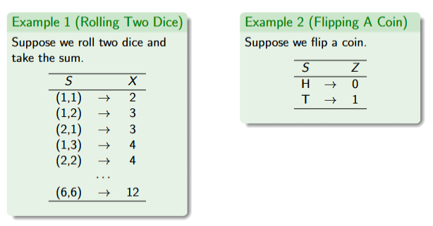
Random Vairable

Numerical measurement of the outcome of an experiment

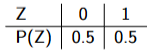
Probability Distribution

Discrete Random Variables

Random Vairable - X

Value - x

Plotted iwth Barplots

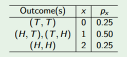
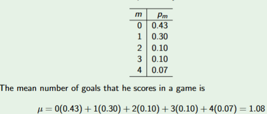
Mean of Discrete Random Variable

Weighted average of the values in the sample space, Expected value.

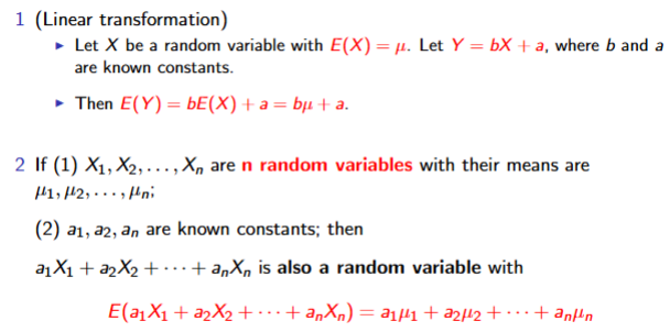
Properties of Mean

1. Linear Transformation

2. Multiple Random Variable Add Mean

3. Mean of random variables is mean

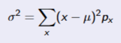
Variance of Discrete Random Variable

\sigma is the standard deviation of X

P is the probability

x is the value

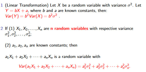
Properties of Variance

1. Multiplication

2. Random Variables Addition works

3. Mean variance of random variables is \sigma/ n

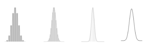
Continous Random Variable

Contains values that form an interval.

Probability Density function area should be less than 1.

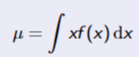
Mean of Continous Random Variable

Expected value of X

Same properties as mean for discrete case

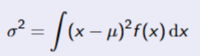
Variance of Continous Random Variable

Same properties as variance of discrete case

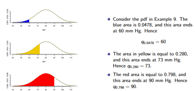
Quantiles of Continous Random Variable

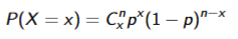
Binomial Distribution (X ~ Bin(n,p))

1. Strictly 2 outcomes

2. Constant probability of success

3. N Trails are independent

4. Mean = NP

5. Variance = NP(1-P)

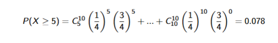
Binomial Distribution Example

Assuming Probability = ¼

N = 5

X = 10

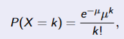
Poisson Distribution

\lambda is the expected number of events over time period t

Poisson can be use to accurately approximate binomial with large n and small p given mean = np

np almost equal to np(p-1)

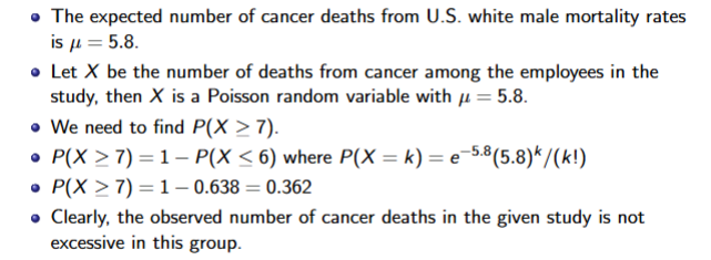
Poisson Distribution Example

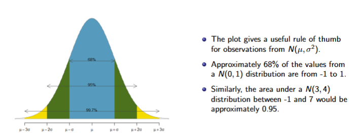
Normal Distribution

1. Symmetric, bell curved and characterised by mean and variance

2. Highest point is at mean

3. SD Diff: 68%, 95%, 99.7%

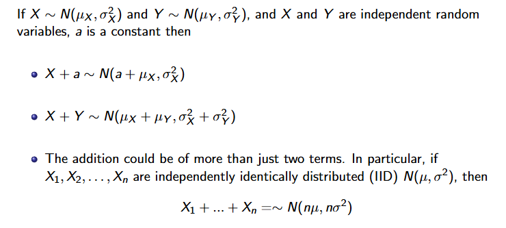
Linear Transformation of Normal Random Variables

• Adding constants forms new variable

• Sum of normal is still normal

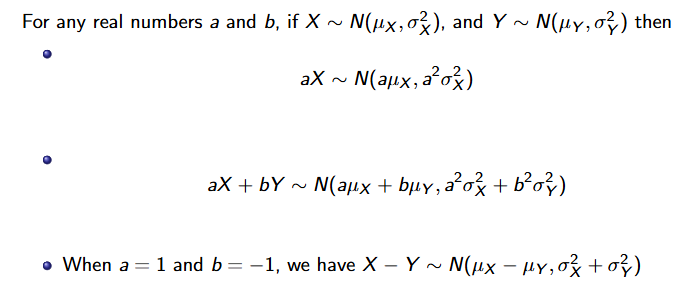
• Product of normal with constant is still normal

Adding Normal Varible

Mutiplying Normal Variable

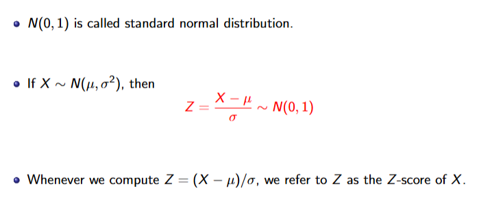
Standard Normal Distribution

N(0,1)

If Z-score is more than 3 or lesser than -3 its a outlier