Lecture 09: Multi-species Interactions and Food Webs

From Individuals to Populations to Communities and Ecosystems

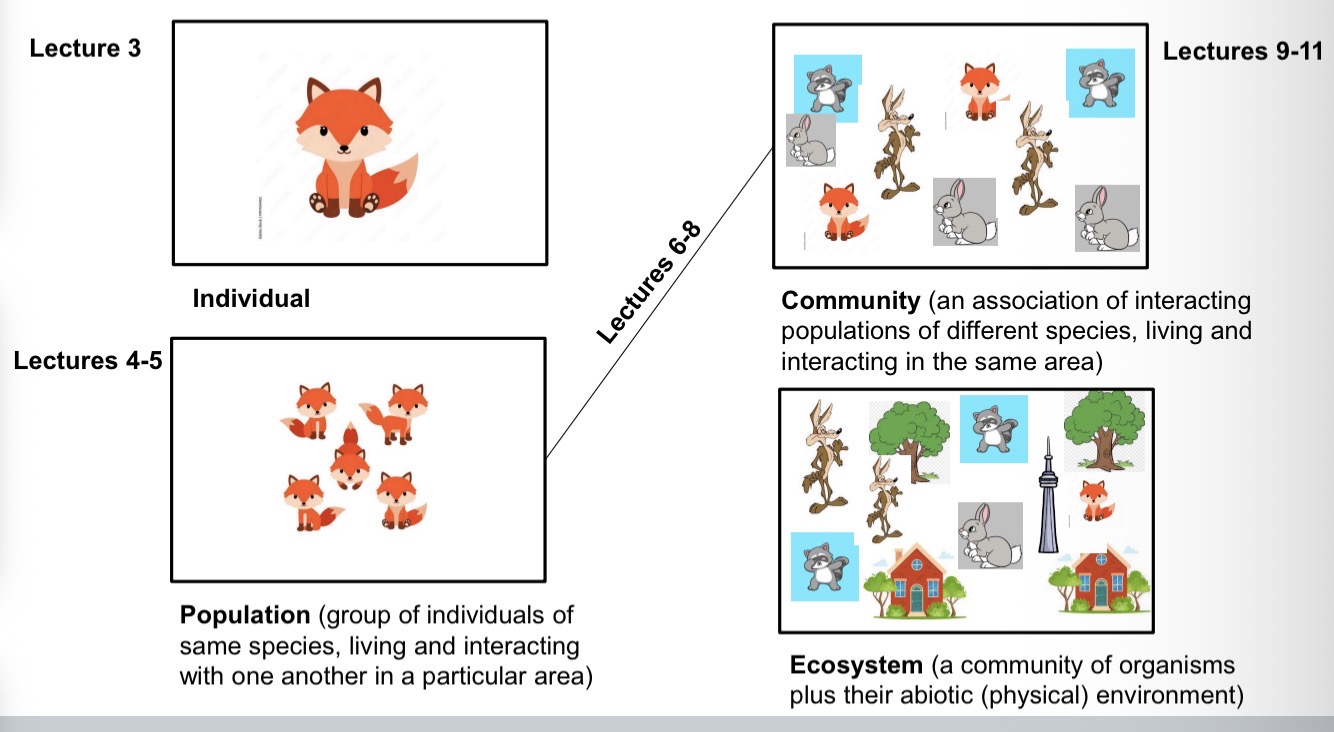
A Puzzle Is More Than Its Parts:

• In communities, multiple populations interact with one another and influence each other’s population dynamics.

• The multitude of interactions necessitates a new perspective and new approaches compared to those that we have discussed in population ecology.

• Nothing is at simple as we have a bunch of levels and everyone just eats the lower levels

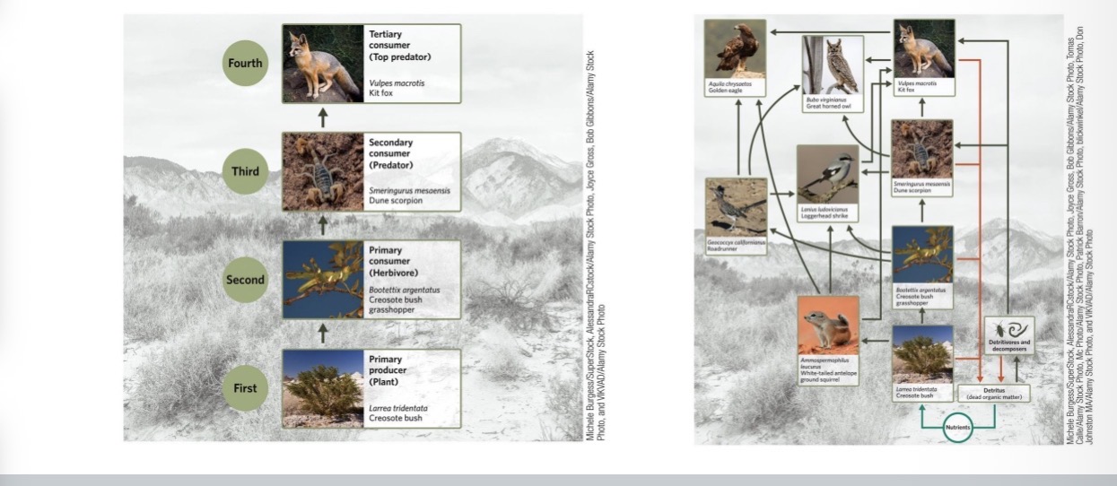
Food chains

• provide a simple conceptual model for energy flows in a community.

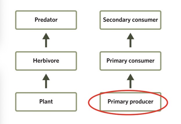
• They depict trophic interactions and simplify community dynamics by sorting species into clearly defined trophic levels.

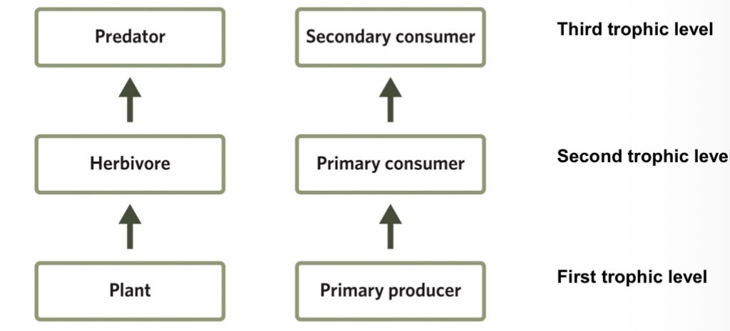
First trophic level

Plant or primary producer

Second trophic level

Herbivore or primary consumer

Third trophic level

Predator or secondary consumer

Examples of food chains

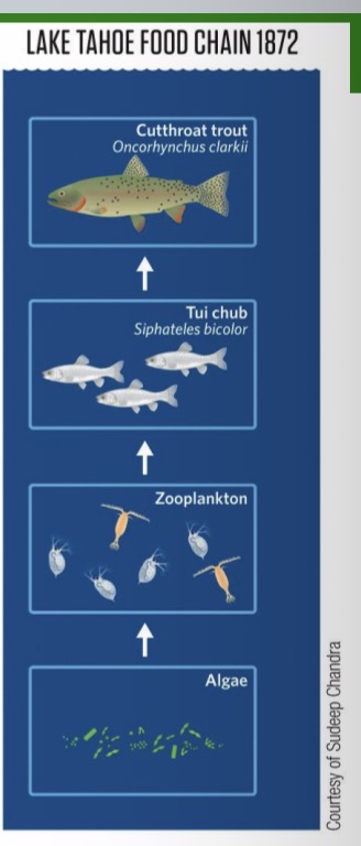
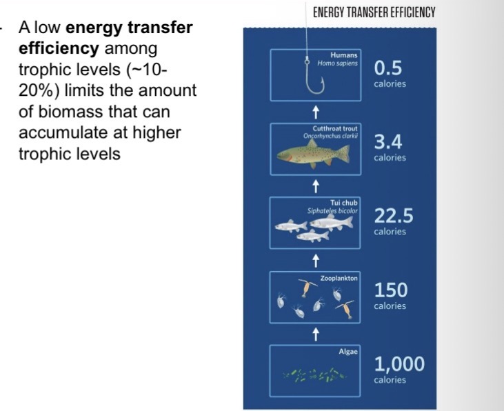
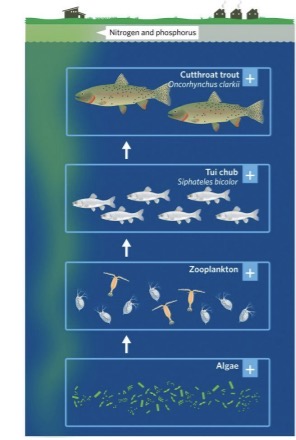
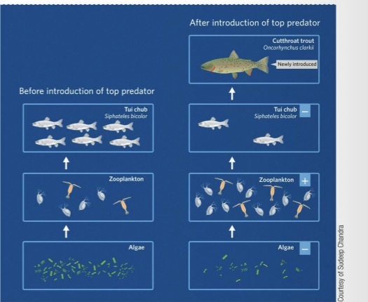
• Example: Lake Tahoe food chain in 1872

  • Obviously no species called algae, thats many species we grouped together. Zooplankton are grouped to one trophic level thats actually many species

Trophic Energy Transfers

• The amount of energy that can be transferred among trophic levels is limited at every step

  • The amount of energy that primary producers can capture via photosynthesis is limited by the availability of sunlight, water, CO2, and other variables.

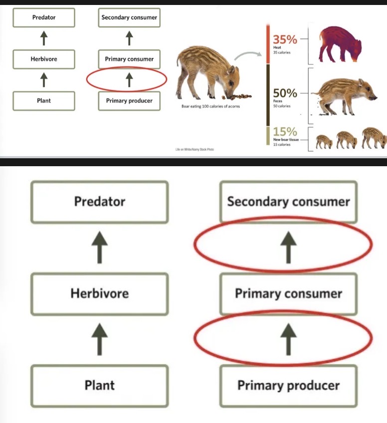
  • Energy transfer can never be perfectly efficient. Energy will dissipate somehow

• However much energy sits at the bottom (primary producers) it will be less in the next level, and even less the level above that

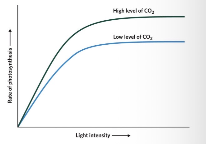
The amount of energy that primary producers can capture via photosynthesis is limited by

• the availability of sunlight, water, CO2, and other variables.

  • If you have low light (dark forest) → low photosynthesis

  • To at canopy (where all light is) → high photosynthesis

  • But at some point it will all level out, you cannot increase photosynthesis infinitely

Why are there more spiders than lions

• In order to get same amount of lions, you need all that energy transferred up the food chain without any loss whatsoever

• Also lions are bigger than spiders so you will get less lions than spiders if energy transfer is 100% efficient, but we get even less lions because energy transfer efficiency is less than 100%

A low energy transfer efficiency among trophic levels

(~10-20%) limits the amount of biomass that can accumulate at higher trophic levels

By the time you get to 4th or 5th trophic levels

Little energy actually remains

Trophic Pyramids

Limits on trophic energy transfer efficiency lead to trophic pyramids that can equivalently be expressed as the amount of energy or the amount of biomass contained within each trophic level

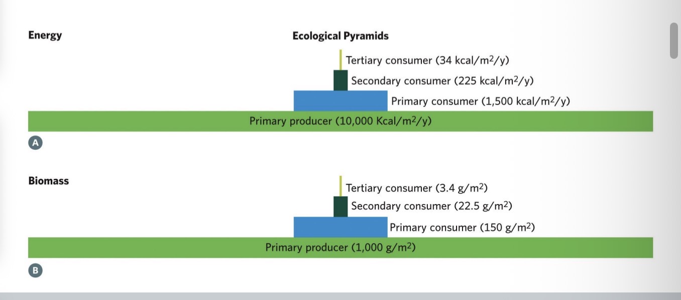
The shape of trophic pyramids can be influenced by the rates of turnaround at each trophic level.

• Aquatic trophic pyramids, for example, often display a lower biomass of phytoplankton (primary producers) than zooplankton (primary consumers) at any given point in time.

• However, phytoplankton have such short lifespans and fast reproduction rates that their biomass still adds up to well more than the biomass of primary consumers when viewed over the entirety of the primary consumer’s generation time

• It’s like saying “im going to give you a batch of cookies” and you would think “well this batch is not enough for my whole life” but then i say “well I’ll give you another batch one second later, and another and another”

  • In one moment in time 1 batch doesn’t look like enough but because the energy source is being replaced so quickly, it is enough

As a consequence of the limited trophic energy transfer efficiency

• most food chains are limited to six trophic levels or less

• Example: Top predators occur at much lower densities than lower trophic levels due to the limits in energy transfer efficiency. A hypothetical predator of such top predators would have to cover huge distances and expend large amounts of energy to sustain themselves (imagine how much energy a hypothetical predator of a lion would need to prey on such a species) Such amounts of energy are not available at upper trophic levels

Considering the limited trophic energy transfer efficiency can reveal unexpected ecosystem connections

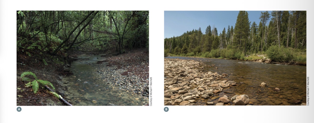
• For example, many ecosystems are supported by both endogenous and exogenous energy inputs.

• Example: Lotic ecosystems subsidized by terrestrial energy inputs

  • Rivers have almost no minerals so they should not be able to support much life. But trees’ leaves fall into water, rot, and bring in energy that way → this is exogenous energy output (energy from outside the system)

Coastal ecosystems subsidized by marine energy inputs

• Let’s imagine we lost all the salmon in BC.

• marine and terrestrial animals would be affected

  • Bears don’t get enough food, their population might go down

  • When salmon die, and their bodies are often dragged onto the forest floor by predators and scavengers like bears, eagles, and wolves. These animals leave uneaten parts of the fish, as well as their droppings, which deposit the marine nutrients into the soil. Without these, the tree growth decreases

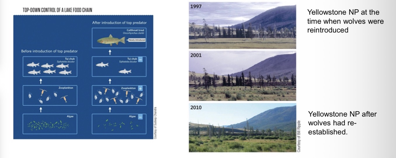
As a consequence of the limited trophic energy transfer efficiency, top predators require large home ranges, posing challenges for conservation efforts.

• Wolf reintroduction in Yellowstone National Park

  • Wolves are top predator and need to roam to get their prey (elk)

  • Yellowstone is 100km by 100km, in that region there were 8-9 wolf packs introduced, and given the limitations of the area, thats good. In fact they start branching outside of Yellowstone because the land is not enough

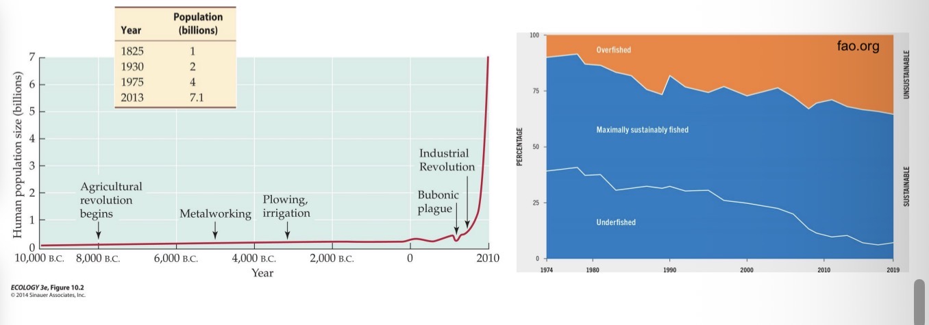
As a consequence of the limited trophic energy transfer efficiency, top predators require large amounts of food to sustain large populations, posing challenges for human food security.

• For a human to persist, you need large area to produce food each of us needs

• We have increased population sizes, so we are running into problem of where will all the food we need come from

• Concerns about

  • Fish that are needed to be taken out of ocean to feed us → overfishing problem

What controls abundance/biomass at each level?

• Bottom up control

• top down control

Bottom-Up Control:

• Control of the energy flow in a food web by organisms at the basic trophic level (autotrophs).

• The abundance of autotrophs limits the amount of energy that is available to, and thus, the abundance of, species at higher trophic levels.

Top-Down Control:

• Control of the energy flow in a food web by organisms at the upper trophic levels.

• By eating organisms at the lower trophic levels, the species at the upper trophic levels control the biomass and abundance of lower levels

• Lots of trout → eat and deplete level below them → fewer tui chub → so now next level is relieved of some predation → lots of zooplankton that will eat more phytoplankton → less phytoplankton

• Odd # of levels (e.g., 3: predator → herbivore → plant):

  • → Top predator ↓ herbivores → ↑ plants

  • Yayyy for Primary producers increase

• Even # of levels (e.g., 4: top predator → mid predator → herbivore → plant):

  • → Top predator ↓ mid predator → ↑ herbivores → ↓ plants

  • BAD for Primary producers decrease

• Summary:

  • Odd = Positive effect on plants

  • Even = Negative effect on plants

Odd # of levels (e.g., 3: predator → herbivore → plant):

• → Top predator ↓ herbivores → ↑ plants

• Yayyy for Primary producers increase

• Tui chub deplete zooplankton → lots of phytoplankton

Even # of levels (e.g., 4: top predator → mid predator → herbivore → plant):

• → Top predator ↓ mid predator → ↑ herbivores → ↓ plants

• BAD for Primary producers decrease

• Ex Lots of trout → eat and deplete level below them → fewer tui chub → so now next level is relieved of some predation → lots of zooplankton that will eat more phytoplankton → less phytoplankton

The effects of bottom-up control can often be seen by

• enriching the lowest trophic level and observing the effects on biomass across upper trophic levels.

• Example: The addition of nutrients to aquatic ecosystems, for example through agricultural fertilizer runoffs, can turn oligotrophic water bodies (few primary producers, low biomass) into eutrophic ones (many primary producers, high biomass

oligotrophic water bodies

few primary producers, low biomass

eutrophic water bodies

many primary producers, high biomass

Bottom-Up Control of Ecosystems: Eutrophication in the Anthropocene

• David Schindler’s “whole-lake-experiment”

  • The amount of nutrients present in lakes can determine the state of an aquatic body. Increasing limiting nutrients, such as phosphorus (P) and nitrogen (N), for example, through fertilization, can result in massive algal blooms.

  • Decomposition of these algae by bacteria depletes the dissolved oxygen in the water and can lead to hypoxia and high zooplankton & fish mortality

  • Some of the nutrients that were added to soils through fertilization will wash into rivers and accumulate downstream (at mouth of river), leading to increased eutrophication, and in some cases, large “dead zones” with little life

Why when there is increased eutrophication there are large “dead zones” with little life

• Because there will be so much algae, it will take all the O2, so not enough O2 left for other things, and fish will start dying

• There is still some living things (dont take ‘dead’ too literally) but significantly less then there could be

The effects of top-down control

• have first been outlined by Aldo Leopold and subsequently, Hairston, Smith, and Slobodkin (HSS), based on the simple observation that the terrestrial world is generally fairly green: what keeps herbivores in check from completely depleting plant biomass?

• HSS suggest that control by competition and predation alternates between trophic levels, with competition controlling the abundance of top predators, predation controlling the trophic level below it, etc

  • If number of levels is even = little primary production

  • If number of levels is odd = lot of primary production

HSS hypothesis (Hairston, Smith, and Slobodkin, 1960), also known as the “Green World Hypothesis.”

• In an ecosystem, the forces that control population sizes (competition vs. predation) alternate between different trophic levels (producers, herbivores, carnivores, etc.).

• How it works:

  • Top predators (like lions) are limited mainly by competition with each other (because they have few natural enemies).

  • The level below them (herbivores) is controlled by predation — predators eat them, keeping their numbers in check.

  • Plants (the next level down) are then controlled by competition for light, water, and nutrients, because herbivores are kept in check by predators — so plants are not eaten to extinction, and the “world stays green.”

• In short : Control alternates like this — Competition → Predation → Competition → Predation, starting from the top of the food chain.

Top-Down Control for Ecosystems: Food Chains with Odd vs Even Numbers of Trophic Levels

Top-down control implies that food chains with odd numbers of trophic levels have high densities of primary producers (a green world), while food chains with even numbers of trophic levels have low densities of primary producers (a brown world).

Summary odd numbers of trophic levels

have high densities of primary producers (a green world)

Summary even numbers of trophic levels

have low densities of primary producers (a brown world)

Top-down and bottom-up control

• typically act simultaneously in ecosystems.

• The combination of their respective contributions determines biomass at each trophic level

Short answer Food Chain:

• is the linear sequence of organisms through which energy and nutrients flow in an ecosystem — each organism feeds on the one below it.

• Example: Grass → Grasshopper → Frog → Snake → Hawk

Short answer Trophic Energy Transfer Efficiency:

• is the percentage of energy that is passed from one trophic level to the next in a food chain.

• Typically, only about 10% of the energy is transferred; the rest is lost as heat, waste, or used for metabolism.

Short answer Top-Down Control:

• occurs when predators (higher trophic levels) regulate the abundance or behavior of organisms at lower trophic levels.

• Example: If wolves reduce deer populations, which then allows more vegetation to grow.

Short answer Bottom-Up Control:

• happens when the availability of resources (like nutrients, sunlight, or water) at the lowest trophic level (producers) determines the structure and productivity of the entire food web.

• Example: More nutrients in soil → more plants → more herbivores → more predators.

The data in the top figure show a decline in shark abundances along the east cost of the United States from the 1970s to the mid-1990s, along with a concordant increase in mesopredators and a decline in scallop abundances. Do the shown data indicate top-down or bottom-up control? Why?

• Top down control

• This sequence — fewer sharks → more rays → fewer scallops — indicates that the abundance at lower trophic levels is being regulated by predation from higher levels.

• That’s top-down control, because:

  • When the top predators (sharks) decline, their prey (rays) are released from predation pressure and their populations grow.

  • The rays, in turn, overconsume their prey (scallops), causing scallop declines.

  • This shows a cascade effect initiated from the top of the food web downward.

If this were bottom up then we would see

• starts with changes at the base of the food web — like nutrients, light, or primary producers (plants/algae).

• If this were bottom-up control, we’d expect:

  • Changes in plankton or vegetation → causing changes in scallops or rays → then finally affecting sharks.

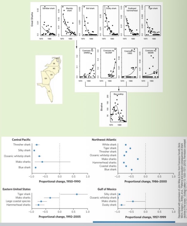
The data in the top figure show a decline in shark abundances along the east cost of the United States from the 1970s to the mid-1990s, along with a concordant increase in mesopredators and a decline in scallop abundances. The bottom figure shows proportional changes in shark abundance by species and region for specified time periods. Describe what trends are seen for the eastern United Stated.

• For the Eastern United States, the data show a strong decline in major shark species — particularly makos, large coastal species and hammerhead— between 1992 and 2005, indicating severe reductions in top predator abundance during that time.

• The dots are to the left of dotted line because relative change means change relative to population size.

  • Makos have decreased less than hammerheads and large coastal species

The data in the top figure show a decline in shark abundances along the east cost of the United States from the 1970s to the mid-1990s, along with a concordant increase in mesopredators and a decline in scallop abundances. How do you think these trends may alter the trends described in the top figure?

• Top one does not show an increase in tigersharks in 1990-2000, but bottom one shows an increase from 1992-2005, both things can be true if increase happened in last few years

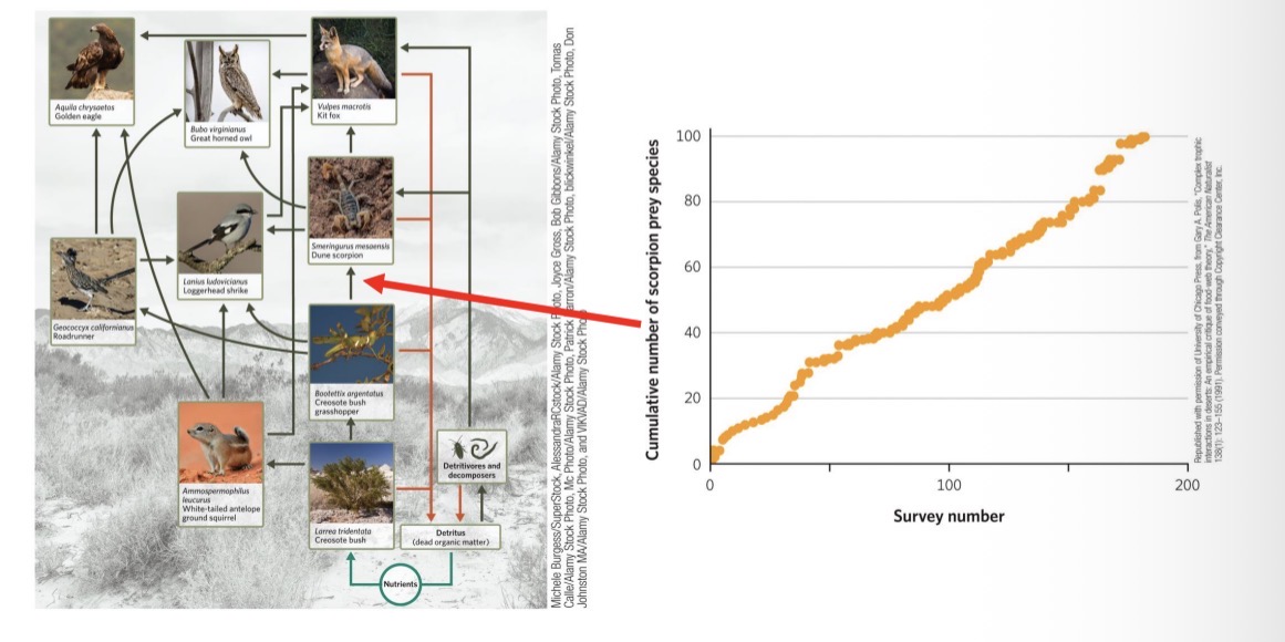
Food chains are simplified representations of reality that omit much biological detail.

They do not distinguish between different species at the same trophic level, omit diet variations (e.g., across seasons or ontogeny), omit multiple feeding interactions both within (e.g., diet variation of a carnivore) and across trophic levels (e.g., omnivory), and omit detritivores and decomposers

How much detail is added depends on

• data availability and the study’s objective.

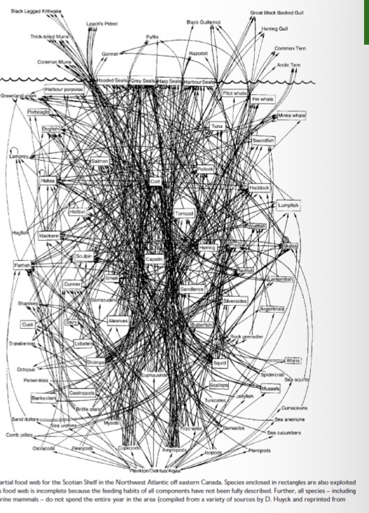
• No matter how much detail is added, a food chain / food web will always underrepresent reality

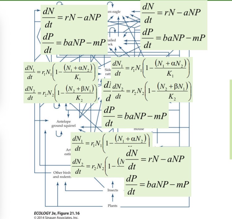
• Ex. Partial food web of the Scotian Shelf in the NW Atlantic Ocean

Partial food web of the Scotian Shelf in the NW Atlantic Ocean

Tons of stuff here that aren’t represented

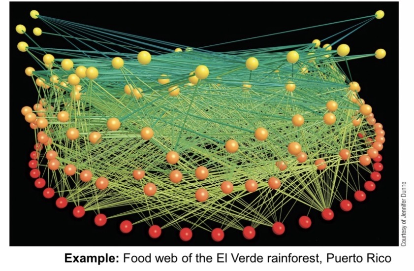
Modern food web diagrams typically use

three-dimensional “ball-and-stick diagrams” to represent the complexity of connections (sticks) among species at various trophic levels (balls; colors indicate trophic levels).

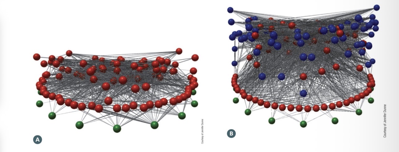
Food web of the Punta Banda marine estuary, Baja California, Mexico, (a) with and (b) without parasites

A specialist parasite that feeds on a lion, has a trophic level above the lion, even though it is smaller

Variation in diet

• makes it difficult to assign a specific trophic level to a species as we have done for food chains.

• Species rarely feed on one trophic level only; quantifying this diet variation is critical for correctly assigning trophic levels

Multiple methodologies exist for determining a species’ diet.

• Direct observation

• Gut content and fecal analyses

• Stable isotopes

Direct observation

was key in many classical studies. However, this method is comparatively inefficient and easily creates documentation biases towards common diet items (what if animal ate something outside the perimeter that was being observed); diet items that are rarely consumed can easily be missed due to limited observation periods

Gut content and fecal analyses

• can provide more complete documentation of a species’ diet, as well as other information such as on the species’ parasites.

• Nevertheless, these methodologies also suffer from similar limitations, and associated biases, arising from difficulties of collecting and analyzing samples as direct observations, including difficulties of tracking rare diet items and diet variation among individuals, life stages, and seasons,

• Ex. White hair in coyote fecus is its prey of deer or boar

Stable isotopes

• are variants of chemical elements that have differing numbers of neutrons in the atomic nucleus that do not decay radioactively over time.

• Using a mass spectrometer, ecologists can measure the ratio of different isotopes in tissue samples (tooth, fur).

• As stable isotopes are preserved through trophic transmission, these ratios can be used to determine an individual’s diet, days, weeks, or even months into the past depending on the tissue sample.

Measuring the carbon isotope ratio 13C:12C in tissue samples can indicate

the source of an individual’s carbon, because different species of primary producers have differing carbon isotope ratio 13C:12C signatures.

Carbon provides

• A fingerprint of what organism has eaten

• Every organism has different carbon signature that gets preserved

• If a bear is eating a seal then those stable isotopes bearing the seals signature will be contained in polar bear as it makes new polar bear in hair, teeth

• Ex. Snail and periphyton have same carbon signature so there must be a feeding relationship (snail ate the periphyton)

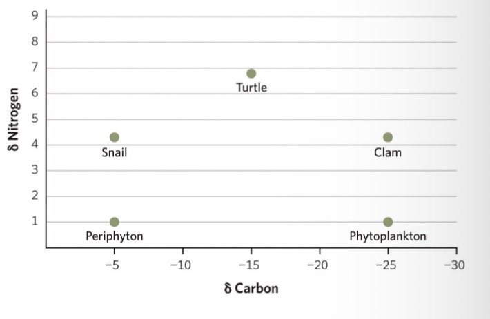
Nitrogen provides

• Accumulates across trophic levels

• Higher up you are on the y axis, the higher the nitrogen signature is, the higher your trophic levels is

• Ex. Turtle is higher trophic level than snail and claim, that are on higher trophic level than periphyton and phytoplankton

Measuring the nitrogen isotope ratio 15N:14N in tissue samples can indicate

an individual’s trophic position, because 15N accumulates in higher trophic levels (~3.4 additional units of 15N per trophic level)

Interaction Webs vs Food Webs

• Despite their complexity, food webs remain simplified representations of reality that omit much biological detail.

• In particular, they do not consider non-feeding interactions or knock-on effects of feeding interactions that ripple through the community. Interaction webs aim to include such interactions in addition to trophic interactions

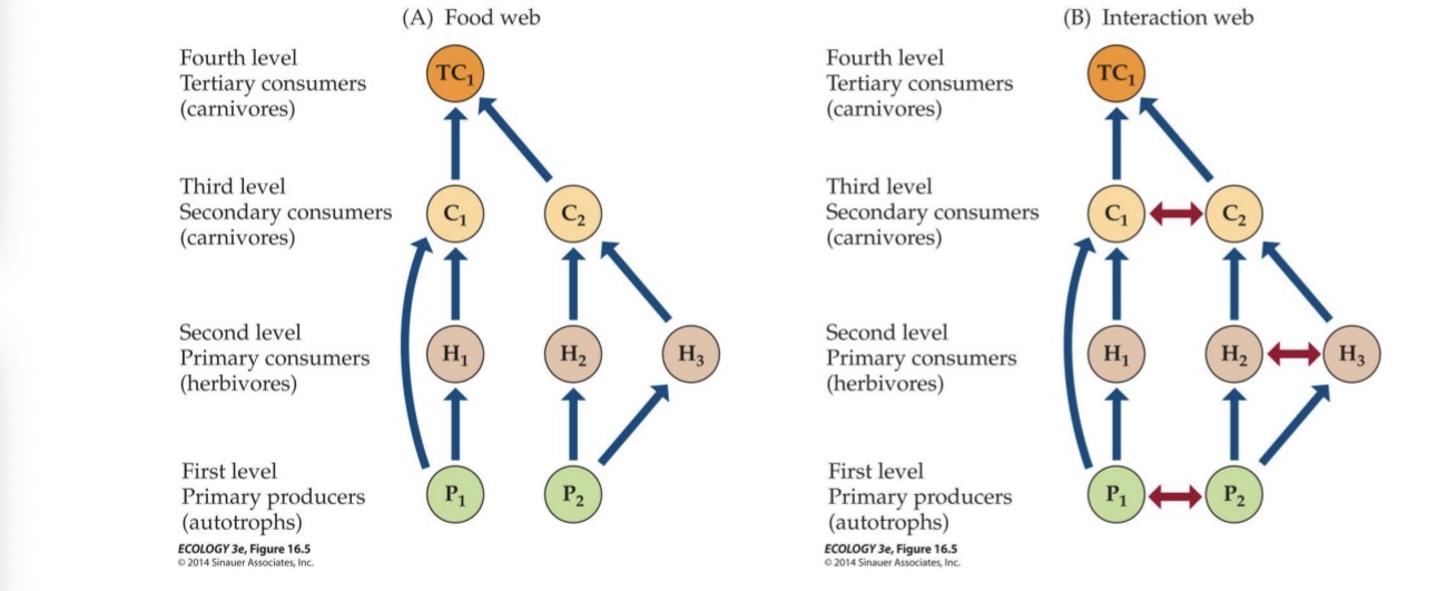
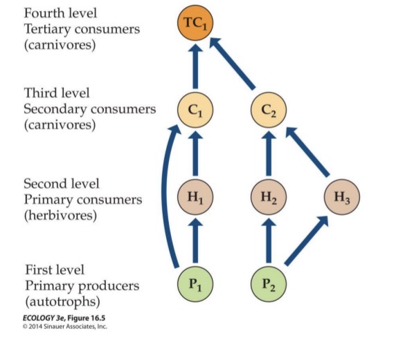
Food webs diagram

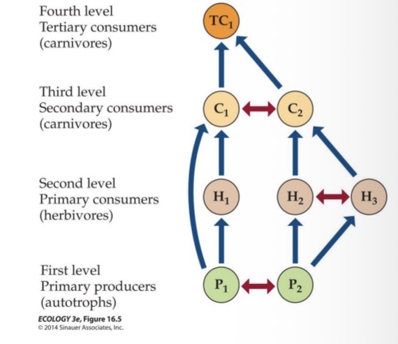
Interaction web diagram

Indirect effects of interactions can substantially influence community function and structure

• Resource competition

• Predator mediated coexistence

• Trophic Casandra

• Apparent competition

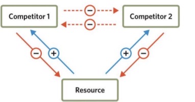
Resource competition

• Often interaction is exploitative where 2 species are eating the same thing. Maybe 1 species is a day time species and the other is a night time species. They exploiting the same food source but at different types so no direct interaction

• (-,-) is indirect because they are eating each others food. Nothing they do to each other directly is negative (they aren’t fighting)

• Competitor → Resource (–)

  Each competitor uses up the resource.

  • So, more Competitor 1 → less Resource.

  • More Competitor 2 → less Resource.

    (That’s why the arrows from Competitors to Resource have “–” signs.)

• Resource → Competitor (+)

  The resource helps both competitors grow.

  • More Resource → more Competitor 1 and Competitor 2.

    (That’s why arrows from Resource to Competitors have “+” signs.)

• Indirect negative effects between competitors (–/–)

  Because both use the same resource, when one competitor increases, it reduces the resource and indirectly harms the other.

  • More Competitor 1 → less Resource → less Competitor 2.

  • More Competitor 2 → less Resource → less Competitor 1.

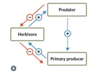
Trophic cascades

• Predator on top, that will have - influence on herbivores (because predators eat herbivores)

• Herbivores will have negative influence on primary producer (because herbivores eat primary producers)

• Less herbivores = more primary producers (indirect + relationship of predators and resource of herbivores)

• Examples: wolves in Yellowstone NP; sea otters & kelp forests

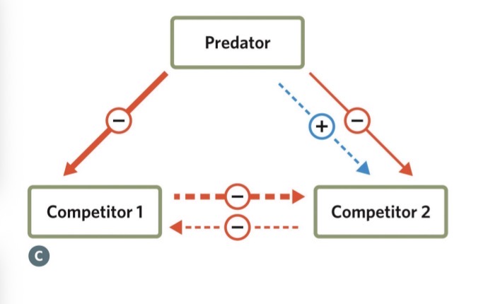
Apparent competition

• Not competition, just appears to be

• 2 species, when both present (example tortoise and mice)

  • When there are more mice = less tortoises

  • Less mice = more tortoises

• Not because of shared food resource

• Explanation is because of predator

  • Lots of tortoises = lots of predator (because they have food to eat) = but now these predators will not just prey on the tortoises but on the mice too = less mice

• abundance of one species is attracting a predator and that predator is also feasting on another species

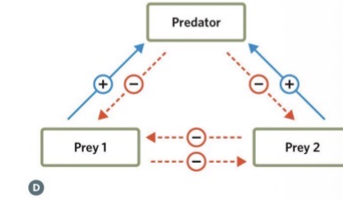
Predatory mediated coexistence

• Competitor 1 or Competitor 2 is much more dominant than the other

• Two species compete for the same resource

  • For example, two kinds of snails both eat seaweed.

  • Species A is stronger and eats faster.

  • Species B is weaker and can’t get enough food.

• Normally, Species A would win, and Species B would disappear.

• Add a predator

  • A crab prefers to eat Species A, the stronger competitor.

• What happens now

  • The predator keeps Species A’s population low.

  • That leaves enough food for Species B too.

  • Both species can now survive together.

• Ex. Predatory sea stars hold highly competitive barnacles in check, allowing a diverse community to thrive

• Ex. tortoises and cactus mice negatively influence each other’s abundances, but this is not through competition for a shared resource but rather through regulation by a shared predator.

Keystone species,

species that have a disproportionately large effect on community structure, function, and/or diversity, relative to their own biomass and/or abundance, and foundation species, i.e., species with a large effect on community structure, function, and/or diversity that is proportional to their biomass and/or abundance

Foundation species are species that

• their impact is proportionate to their size in the ecosystem.

• have a large effect on community structure, function, and/or diversity that is proportional to their biomass and/or abundance

• Ex. Trees in a forest. Without trees you don’t have a forest

Keystone species definition and examples

• are species that have a disproportionately large effect on community structure, function, and/or diversity, relative to their own biomass and/or abundance.

• Take out these species the ecosystem collapse

• Example: Robert Paine originally proposed the idea of keystone species by studying predatory sea stars: when the sea stars were present, highly competitive barnacles were held in check, allowing a diverse community to thrive

• Examples: Many keystone species are predators whose actions keep otherwise dominant species from displacing other species.

• Examples: Many keystone species are mutualists, whose actions support large parts of a community and/or some foundation species. → bees

• Not necessarily abundant

Difference between foundation and keystone species

• Foundation species their impact is proportionate to their size in the ecosystem.

• Keystone species have a disproportionately large effect on ecosystem balance (e.g., wolves, sea stars, sharks). They control populations and maintain biodiversity.

• Foundation = proportionate

• Keystone = disproportionate

The loss of a keystone species can substantially alter the composition and dynamics of communities.

Example: Trophic cascade due to shark removal

Trophic cascade due to shark removal (sharks as a keystone species)

• Removing sharks (the keystone predators) causes a trophic cascade:

• Shark numbers drop → rays and other mesopredators increase → scallops and shellfish decline.

• This shows that the loss of a keystone species can drastically change the composition and balance of an entire community.

Both keystone species and foundation species can be

ecosystem engineers

Ecosystem engineers

• species that create, modify, maintain, or destroy physical habitat.

• Ex. Beavers, elephants uprooting trees, humans and deforestation

Keystone species Summary

= balancer (keeps ecosystem stable)

Engineer species Summary

= modifier (changes the environment’s structure)