ST411 Weeks 3-5: Models for binary response variables, General theory of GLMs, estimation, and inference

What kind of distribution is used for a binary response variable, and how is it defined?

Binary response variable Y_i uses the Bernoulli distribution

Y_i \sim \text{Bernoulli}(\pi_i)

-

\pi_i is the probability of outcome = 1 (success)

\pi_i = P(Y_i = 1)

What is the mean of a Bernoulli-distributed response variable Y_i?

Mean: E(Y_i) = \mu_i = \pi_i

-

\pi_i is the probability of success (i.e. Y_i=1)

What is the variance of a Bernoulli-distributed response variable Y_i?

Variance: \text{var}(Y_i) = \pi_i(1 - \pi_i)  

Why shouldn’t we use linear regression for binary Y?

Normality assumption is inappropriate for binary Y_i

Assumes constant variance \text{var}(Y_i) = \sigma^2

But for Bernoulli, var. depends on variable we’re modelling: \text{var}(Y_i) = \pi_i(1 - \pi_i)

Fitted probabilities \hat\pi_i can be outside [0,1] (impossible)

What is a link function in binary response models generally?

A link function g(\cdot) connects the mean \pi_i of the response variable to the linear predictor.

Model: g(\pi_i) = x_i'\beta

Ensures fitted values \pi_i = g^{-1}(x_i'\beta) stay in [0,1]

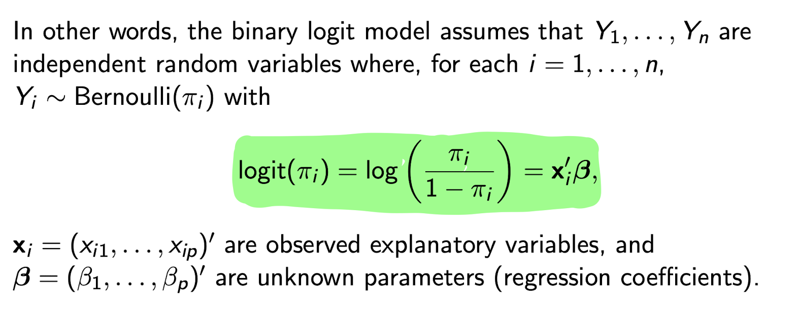
What is the logit link function (forward)?

g(\pi_i) = \log\left(\frac{\pi_i}{1 - \pi_i}\right) = x’_i \beta

-

Also written as \text{logit}(\pi_i)

\pi_i / (1 - \pi_i) is the odds of success

This transforms probabilities in (0,1) to the whole real line (-\infty , \infty)

g(\pi_i) = \\pi_i = \frac{\exp(x_i'\beta)}{1 + \exp(x_i'\beta)}$$ es it guarantee?

Inverse link: \pi_i = \frac{\exp(x_i'\beta)}{1 + \exp(x_i'\beta)}

-

Takes the linear combination xi’B and maps it back to probabilities pi. This is usefull when we generated predicted (fitted) probabilities.

Always gives values between 0 and 1

Keeps \pi_i within valid probability range

Binary logit model overview

• NOT written in mean+residual form

• No separate conditional variance parameter \sigma² , and no assumptions about it are needed

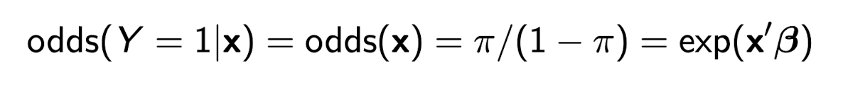
What are the odds that Y=1 in a logit model?

\frac{\pi}{1-\pi}

How do we interpret a coefficient \beta_j in a logistic regression model?

If x_j increases by a units

Then odds of Y = 1 are multiplied by \exp(a\beta_j)

This is the odds ratio comparing two values of x_j

How do we express the percent change in odds when x_j increases by a units?

Percent change in odds: (\exp(a\beta_j) - 1) \times 100\%

If \exp(a\beta_j) > 1, odds increase

If \exp(a\beta_j) < 1, odds decrease

In a logistic regression, what happens if we re-code Y=0 as in favour and Y=1 as against?

It simply reverses the signs of every coefficient. The fit and interpretation remain the same.

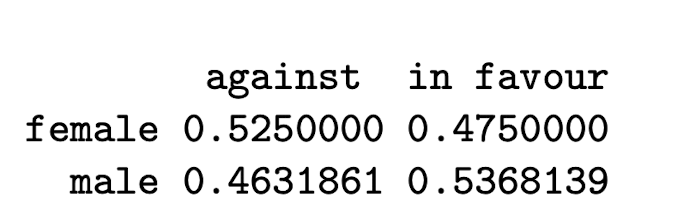
What are the odds a female has Y=1 (is in favour)?

\text{odds}(female) = \pi / (1- \pi) = 0.475/ (1-0.475) = 0.91

What are the odds a male has Y=1?

\text{odds}(male) = \pi / (1- \pi) = 0.537/ (1-0.537) = 1.1598

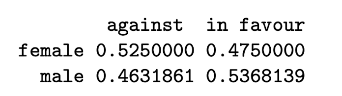
What is the odds ratio for Y=1 (being in favour for basic income) for men vs. women?

The odds ratio is calculated as \frac{odds(male)}{odds(female)} = \frac{1.1598}{0.91} \approx 1.276. It indicates how much more likely men are to be in favor compared to women. This means that the odds of men supporting UBI is are approximately 27.6% higher than female.

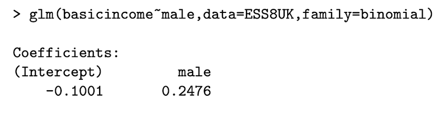
Write out the model for this regression and interpret this coefficient for the UBI example

\log\left(\frac{\pi_i}{1 - \pi_i}\right) = -0.1001 + 0.2476 \cdot \text{male}_i

Men have e^{0.2476} = exp(0.2476) = 1.28 times the odds of supporting basic income compared to women.

Men have 28% higher odds of supporting basic income than women.

Odds of female can be calculated from \beta_0 .

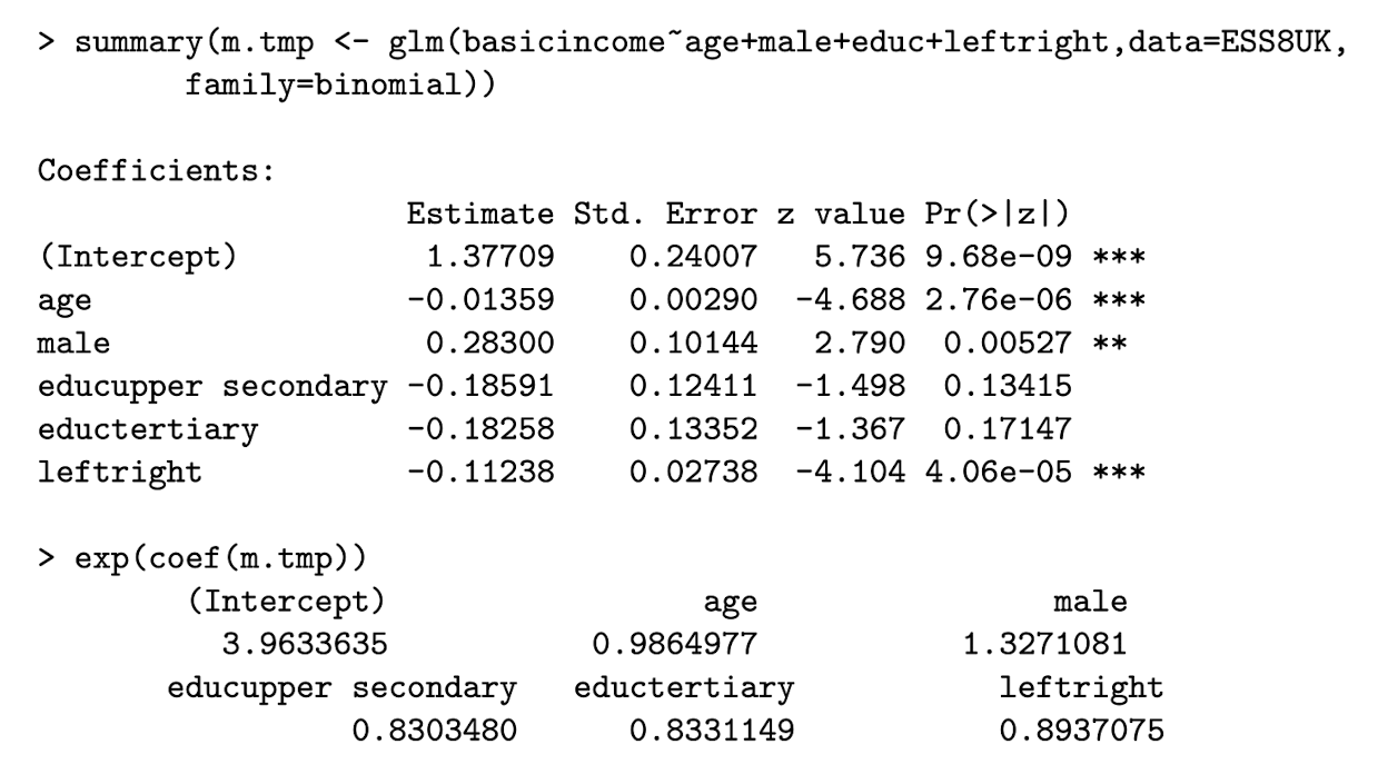
Interpret the coefficient on leftright

leftright is a continuous variable indicating political standing, so be careful.

The negative coefficient indicates that as we increase unit leftright, the odds are reduced.

Controlling for explanatory variables, increasing leftright by one unit, while holding all other variable constant, is associated with a odds in favour being multiplied by e^-0.11 =0.89 .

Controlling for other explanatory variables, a one-point increase in leftright is associated with a 11% reduction in the odds of supporting basic income.

Interpret the coefficient on educupper secondary

Having an upper secondary education (relative to lower secondary) multiplies the odds of supporting basic income by e^{-0.186} = 0.83 , holding all other explanatory variables constant.

This means that individuals with upper secondary education have 17% lower odds of supporting basic income compared to those with lower secondary education holding all other explanatory variables constant.

Interpret the coefficient on age

Controlling for gender, education, and political standing, a one-year increase in age is associated with a e^{-0.014} = 0.986 multiplies the odds of supporting basic income by 0.986.

Controlling for gender, education, and political standing, a one-year increase in age is associated with a 1.4% decrease in the odds of supporting basic income.

What is the formula for the fitted probability \hat\pi(x) in a logistic regression model?

\hat\pi(x) = \frac{\exp(x'\hat\beta)}{1 + \exp(x'\hat\beta)}

-

x is a covariate vector

\hat\beta is the vector of estimated coefficients

\hat\pi(x) is the predicted probability that Y = 1

What are two common ways to interpret fitted probabilities \hat\pi(x)?

1. Change one variable in x and keep others fixed, see how \hat\pi(x) changes

2. Set one variable to the same value for everyone, keep others as they are, average the \hat\pi(x_j) across all units.

   1. Example:

      Set education = college for everyone

      Keep age, income, etc. as observed

      Average the predicted probabilities

      Shows expected probability if everyone had a college degree

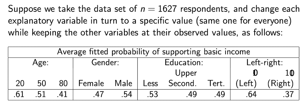
Interpret the predicted probabilities

When we fix age and keep all other variables as-is, when we move from Age = 20 to Age = 50, there is a 0.2 pp decrease in probability of supporting basic income.

-

When we fix gender and keep all other variables as-is, when we move from female to male, there is a 0.07 pp increase in probability of supporting basic income.

-

…

-

Highest differences in Age and Left-Right (-0.27). So these variables are more strongly associated with differences in levels of support for basic income than are gender and education.

Linear model as a GLM: (1) write the distribution, (2) the (linear) predictor, and (3) the link function.

1. Y_i \sim N(\mu_i, \sigma^2)

Response follows a normal distribution

Mean \mu_i, constant variance \sigma^2

-

2. \eta_i = x_i'\beta

Linear predictor \eta_i is a linear combination of covariates

-

3. g(\mu_i) = \eta_i

Link function is the identity: g(\mu) = \mu

Connects mean \mu_i to the linear predictor

Binary logit model as a GLM: (1) write the distribution, (2) the (linear) predictor, and (3) the link function.

1. Y_i \sim \text{Bernoulli}(\mu_i)

Binary outcome with mean \mu_i = \pi_i = E(Y_i)

-

2. \eta_i = x_i'\beta

Linear predictor \eta_i is the same form as in all GLMs

-

3. g(\mu_i) = \eta_i

Link function is the logit: g(\mu) = \log\left(\frac{\mu}{1 - \mu}\right)

Links the mean to the linear predictor using a logistic transformation

What are the three key components of a Generalized Linear Model (GLM)?

1. Y_i follows a distribution in the two-parameter exponential family

Mean is \mu_i = E(Y_i)

-

2. \eta_i = x_i'\beta

Linear predictor from covariates and coefficients

-

3. g(\mu_i) = \eta_i

Link function g(\cdot) connects the mean to the linear predictor

-

Different GLMs use different combinations of distribution and link function

What is the two-parameter exponential family?

Models that include:

1. Mean-related parameter (often the mean)

2. Dispersion parameter (often the variance)

“Exponential family” comes from the fact the PDF function of the distributions can be written in an exponential form.

What are the properties of a link function?

Should be monotonic

Should be differentiable

Should map the range of \mu to valid values for all \eta

Example: probabilities need \mu \in [0, 1]

Example: positive outcomes need \mu \in (0, \infty)

What does it mean for a distribution to be in the exponential family?

A distribution belongs to the exponential family

if its log-density can be written as:

\log f(y; \theta) = \sum_{j=1}^{k} \eta_j(\theta) T_j(y) - A(\theta) + d(y)

-

This is a general form that includes many common distributions

Works for both discrete and continuous outcomes

What are the parts of the exponential family form?

\eta_j(\theta) = natural parameters - depend on the model parameters

T_j(y) = natural statistics - depend on the observed data

A(\theta) = normalizing function (makes density integrate to 1)

d(y) = function of data only

The case of two-parameter exponential family we focus on in this course

Log-density written as:

\log f(y; \theta, \phi) = \frac{y\theta - b(\theta)}{\phi} + c(y; \phi)

\theta = canonical (mean-related) parameter

\phi = dispersion (variance-related) parameter

b(\theta) = known function of \theta

c(y; \phi) = function of data and \phi only

What types of distributions are included in the two-parameter exponential family?

Normal

Binomial

Poisson

Gamma

-

Used for both continuous and discrete data

How do we find the mean of a two-parameter exponential family distribution?

\mathbb{E}(Y) = \mu = b'(\theta)

-

Take the first derivative of the function b(\theta)

This gives the expected value of Y

How do we find the variance of a two-parameter exponential family distribution?

\text{var}(Y) = \phi \cdot b''(\theta)

-

Take the second derivative of b(\theta)

Multiply by the dispersion parameter \phi

What is the variance function in a two-parameter exponential family?

Variance is written as: \text{var}(Y) = \phi \cdot V(\mu)

Where V(\mu) = b''(\theta)

-

This is called the variance function

It shows how variance depends on the mean \mu

What does it mean to use the canonical link function in a GLM?

Set the link function g(\mu_i) equal to the natural parameter \theta(\mu_i)

So that:

g(\mu_i) = \theta(\mu_i) = \eta_i = x_i'\beta

This choice is called the canonical link function

Show that the normal distribution is part of the two-parameter exponential family. Also write out the canonical and dispersion parameters, the mean, and the variance.

Start with the pdf:

f(y; \mu, \sigma^2) = \frac{1}{\sqrt{2\pi\sigma^2}} \exp\left(-\frac{1}{2} \left(\frac{y - \mu}{\sigma} \right)^2\right)

-

Take the log and rearrange:

\log f(y; \mu, \sigma^2) = \frac{y\mu - \mu^2/2}{\sigma^2} - \frac{1}{2} \log(2\pi\sigma^2) - \frac{y^2}{2\sigma^2}

This matches the two-parameter exponential family form:

\log f(y; \theta, \phi) = \frac{y\theta - b(\theta)}{\phi} + c(y; \phi)

-

Canonical parameter: \theta = \mu

Dispersion parameter: \phi = \sigma^2

Function b(\theta) = \mu^2 / 2

Function c(y; \phi) = -\frac{1}{2} \log(2\pi\sigma^2) - \frac{y^2}{2\sigma^2}

-

Mean: \mathbb{E}(Y) = b'(\theta) = \mu

Variance: \text{var}(Y) = \phi \cdot b''(\theta) = \sigma^2

Show that the Bernoulli distribution is part of the two-parameter exponential family. Also write out the canonical and dispersion parameters, the mean, and the variance.

Start with the pmf:

f(y; \pi) = \pi^y (1 - \pi)^{1 - y}

-

Take the log and rearrange:

\log f(y; \pi) = y \log\left(\frac{\pi}{1 - \pi}\right) + \log(1 - \pi)

-

This matches the exponential family form:

\log f(y; \theta) = y \theta - b(\theta) + c(y; \phi)

-

Canonical parameter: \theta = \log\left(\frac{\pi}{1 - \pi}\right)

Dispersion parameter: \phi = 1 (no separate dispersion)

Function: b(\theta) = \log(1 + e^\theta)

Function: c(y; \phi) = 0

-

Mean: \mathbb{E}(Y) = b'(\theta) = \frac{e^\theta}{1 + e^\theta} = \pi

Variance: \text{var}(Y) = \phi \cdot b''(\theta) = \pi(1 - \pi)

what do we use a likelihood function for?

To estimate unknown parameters \theta from data

Helps us find the values of \theta that make the observed data most likely

Used in maximum likelihood estimation (MLE)

Also used for inference (e.g. confidence intervals, likelihood ratio tests)

What is the likelihood function for independent random variables, and how is it defined?

Let Y = (Y_1, \dots, Y_n) be independent random variables

Each has density f(y_i; \theta)

Then the likelihood function is:

L(\theta; y) = \prod_{i=1}^n f(y_i; \theta)

It's a function of the parameter \theta given the data y

What is the log-likelihood function and how is it written?

Take the log of the likelihood:

\ell(\theta; y) = \log L(\theta; y) = \sum_{i=1}^n \log f(y_i; \theta)

This simplifies products into sums

Each term \ell(\theta; y_i) is the log-likelihood for one observation

Transform the likelihood function into the log-likelihood.

Likelihood:

L(\theta; y) = \prod_{i=1}^n f(y_i; \theta)

-

Log-likelihood:

\ell(\theta; y) = \log L(\theta; y) = \sum_{i=1}^n \log f(y_i; \theta)

-

Turns products into sums

Makes optimization easier

in plain english, describe what l(theta; y_i) represents

It’s the log-likelihood contribution from a single observation y_i

Tells us how well the parameter \theta explains that one data point

Part of the total log-likelihood, which adds up contributions from all observations

What is a maximum likelihood estimate (MLE)?

An MLE is the value of \theta that makes the observed data most likely

-

It maximizes the likelihood:

\hat\theta = \arg\max_\theta L(\theta; y)

-

Or equivalently, maximizes the log-likelihood:

\hat\theta = \arg\max_\theta \ell(\theta; y)

How to we find the MLE?

In practice, we find \hat\theta by taking the first derivative of \ell(\theta; y)

. This value is called the score function, which we Set it equal to zero and solve

What is the score function and what is it used for?

The score function is the first derivative of the log-likelihood:

s(\theta; y) = \frac{\partial}{\partial \theta} \ell(\theta; y)

-

Used to find the MLE by solving:

s(\theta; y) = 0

-

The score function depends on the data \mathbf{Y}

So it is itself a random variable

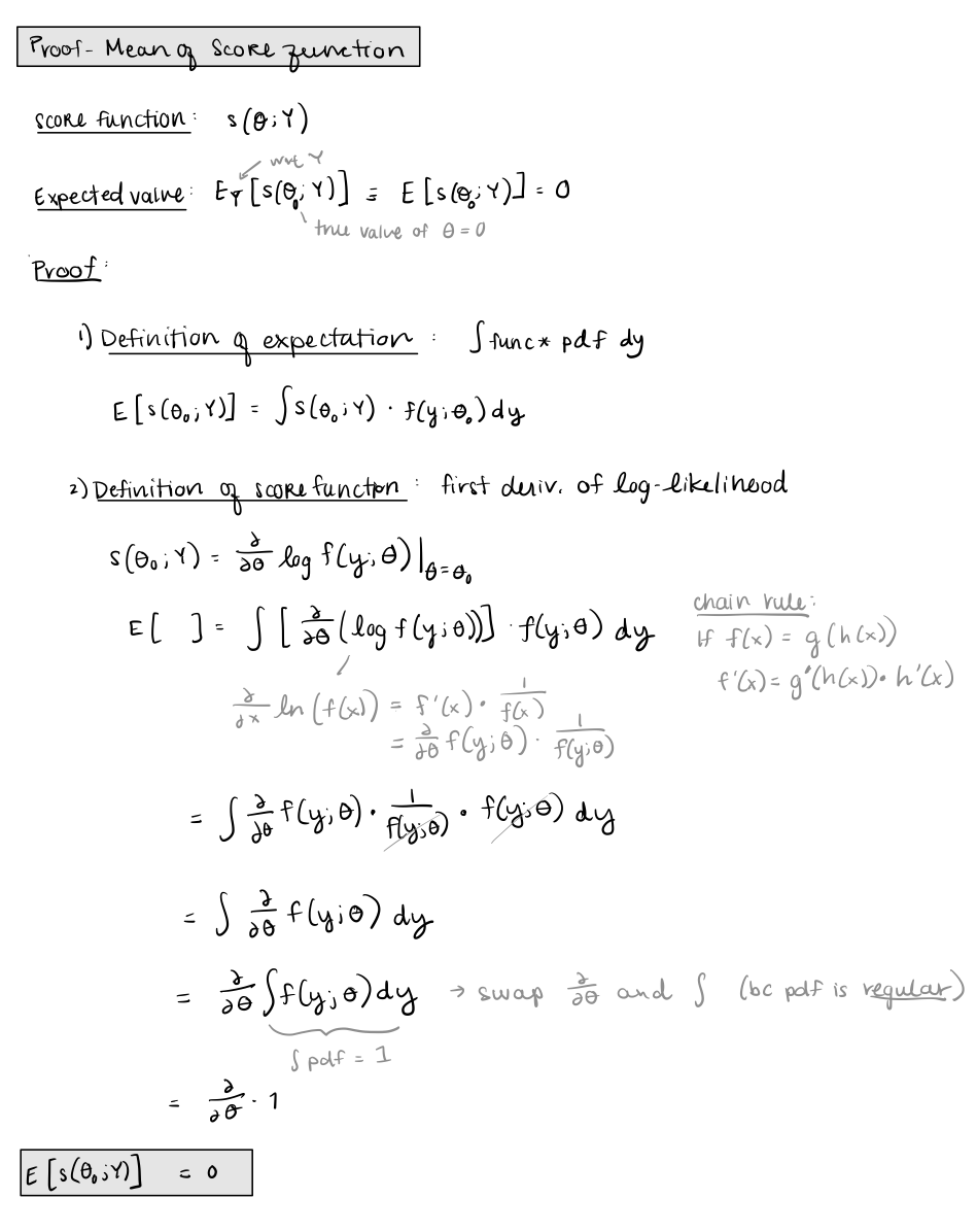
What is the expected value of the score function at the true parameter value \theta_0?

The expected value is zero:

\mathbb{E}_{\mathbf{Y}}[s(\theta_0; \mathbf{Y})] = 0

-

This means the score function has mean zero when evaluated at the true parameter

-

Why:

It comes from:

- Definition of score as a derivative of log-likelihood

- Swapping derivative and integral (regularity condition)

- Total area under pdf is 1, so its derivative is 0

Proof that the mean of the score function is 0

What is the variance of the score function, and what is it called?

The variance of the score function at \theta_0 is the expected Fisher information:

\text{Var}[s(\theta_0; \mathbf{Y})] = \mathbb{E}_\mathbf{Y}\left[s(\theta_0; \mathbf{Y}) s(\theta_0; \mathbf{Y})' \right] = \mathcal{I}(\theta_0)

-

Also written as:

\mathcal{I}(\theta_0) = -\mathbb{E}_\mathbf{Y}\left[\frac{\partial^2 \ell(\theta_0; \mathbf{Y})}{\partial \theta \, \partial \theta'} \right]

-

This is called the expected Fisher information matrix

It equals the negative expected value of the Hessian of the log-likelihood

What happens to the MLE as the sample size grows large?

As the sample size increases, the MLE \hat\theta becomes approximately normal:

\hat\theta \sim N(\theta_0, \mathcal{I}(\theta_0)^{-1})

-

This means:

- It’s approximately unbiased: E(\hat\theta) = \theta_0

- Its variance is the inverse of the Fisher information

-

To estimate the variance, plug in \hat\theta into either:

- the expected information: \widehat{\text{var}}(\hat\theta) = \mathcal{I}(\hat\theta)^{-1}

- or the observed information: \widehat{\text{var}}(\hat\theta) = I(\hat\theta; \mathbf{y})^{-1}

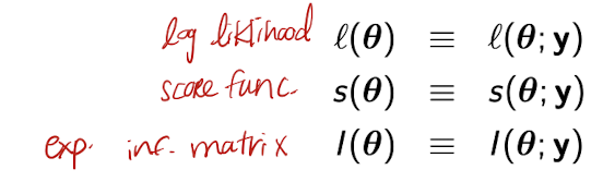
Simplified notation of log likelihood, score func, expected information matrix

What are the key properties of the MLE and the score function?

1. MLE (Maximum Likelihood Estimator):

- Solves the equation: score = 0

- Asymptotically unbiased: E(\hat\theta) \approx \theta_0

- Asymptotically normal: \hat\theta \sim N(\theta_0, \mathcal{I}(\theta_0)^{-1})

- Variance can be estimated using expected or observed information

2. Score Function:

- First derivative of the log-likelihood

- Has mean 0 at the true parameter: \mathbb{E}_Y[s(\theta_0; Y)] = 0

- Variance equals the Fisher information matrix:

\text{Var}[s(\theta_0; Y)] = \mathcal{I}(\theta_0)

3. Information Matrices:

- Expected info: \mathcal{I}(\theta) = -\mathbb{E}\left[\frac{\partial^2 \ell}{\partial\theta \partial\theta'}\right]

- Observed info: I(\theta; y) = -\frac{\partial^2 \ell}{\partial\theta \partial\theta'} at observed y

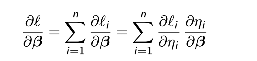
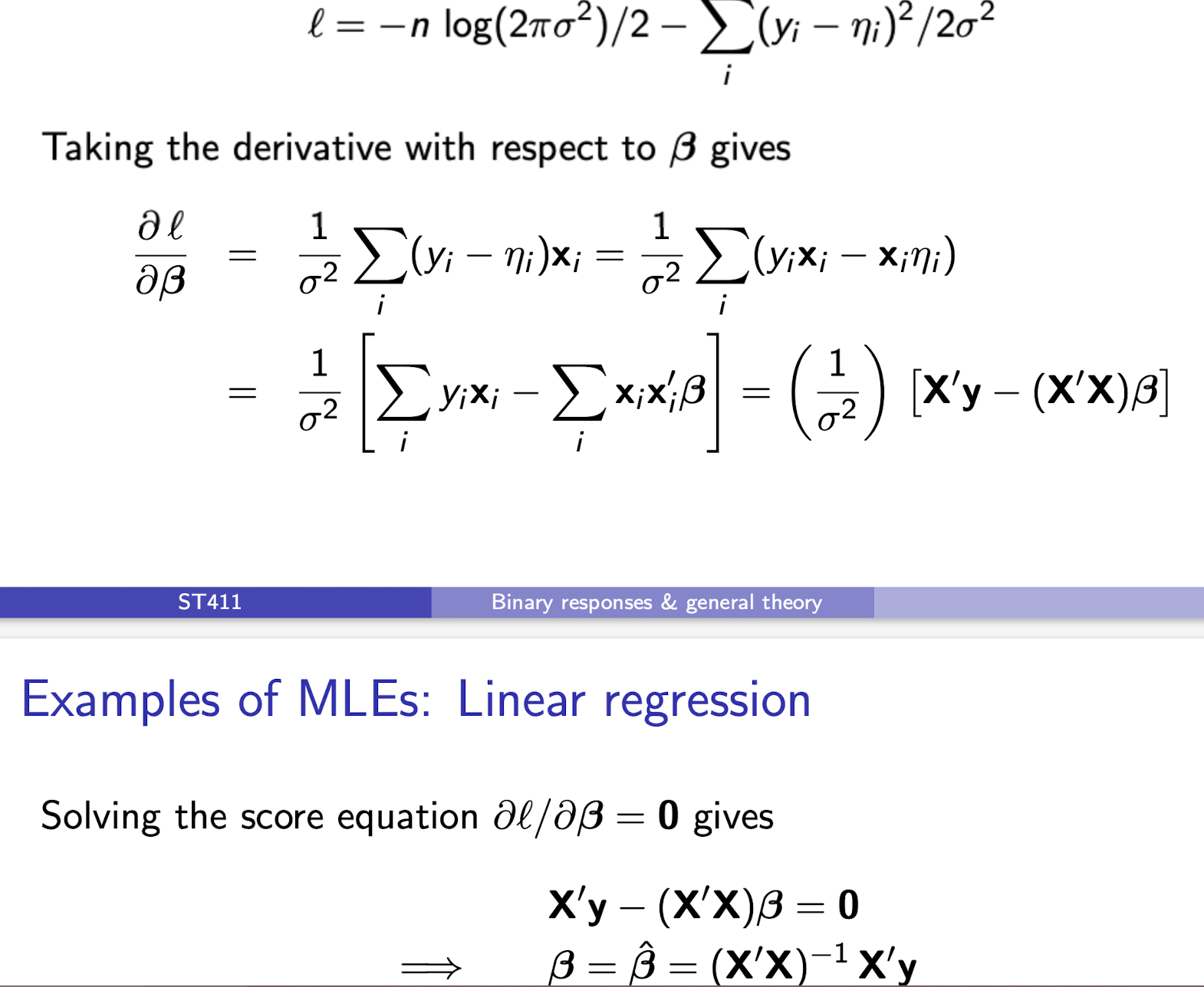
Useful way to take derivatives when finding the MLE

Chain rule of differentiation, using \eta_i because itis a scalar and \frac{\partial \eta_i}{\partial \beta} = x_i always.

Finding the MLE for normal linear regression model

How is \pi related to \beta_0 in the binary logit model with only a constant?

\log\left( \frac{\pi}{1 - \pi} \right) = \beta_0

-

\pi = \frac{e^{\beta_0}}{1 + e^{\beta_0}}

What is the log-likelihood function for the binary logit model with a constant only?

\ell = \sum_i y_i \log\left( \frac{\pi}{1 - \pi} \right) + n \log(1 - \pi)

-

= \sum_i y_i \beta_0 - n \log(1 + e^{\beta_0})

What is the score function (first derivative of the log-likelihood) for the binary logit model?

\frac{\partial \ell}{\partial \beta_0} = \sum_i y_i - n \cdot \frac{e^{\beta_0}}{1 + e^{\beta_0}} = n(\hat{p} - \pi)

What is the MLE of \beta_0 in the binary logit model with only a constant?

\hat{\beta}_0 = \log\left( \frac{\hat{p}}{1 - \hat{p}} \right)

When can the MLE fail to exist in a simple binary logit model?

When certain configurations of x_i and y_i fully separate the data

-

For example, if all y_i = 1 when x_i = 1, the MLE for \beta_1 does not exist

Why do we need iterative methods to find MLEs?

Because for most models, the score equations s(\theta) = 0 cannot be solved analytically

-

They must be solved numerically using iterative methods

What is the first-order Taylor expansion of the score function s(\theta) about \theta_0?

s(\theta) \approx s(\theta_0) + s'(\theta_0)(\theta - \theta_0)

-

Where s'(\theta_0) is the derivative of s(\theta) evaluated at \theta = \theta_0 . \theta_0 is the true value , but is unknown.

What is the Hessian matrix in the multivariate case?

-I(\theta) = \frac{\partial s(\theta)}{\partial \theta'} = \frac{\partial^2 \ell(\theta)}{\partial \theta \partial \theta'}

-

It is the negative of the observed information matrix.

How is the Newton-Raphson approximation for \hat{\theta} derived?

Using s(\theta) \approx s(\theta_0) - I(\theta_0)(\theta - \theta_0)

-

Rearranged at s(\hat{\theta}) = 0 to give \hat{\theta} \approx \theta_0 + I(\theta_0)^{-1} s(\theta_0)

Why can't we use the Newton-Raphson approximation directly?

Because \theta_0 is unknown

-

We must approximate it using iterative updates from an initial value

What is the iterative update formula in the Newton-Raphson algorithm?

\theta^{(m+1)} = \theta^{(m)} + I(\theta^{(m)})^{-1} s(\theta^{(m)})

How does Fisher scoring differ from Newton-Raphson?

It replaces the observed information matrix I(\theta)

-

With the expected information matrix \mathcal{I}(\theta) = \mathbb{E}[I(\theta)]

What is the Fisher scoring update step?

\theta^{(m+1)} = \theta^{(m)} + \mathcal{I}(\theta^{(m)})^{-1} s(\theta^{(m)})

What is the general form of the log-likelihood for a Generalized Linear Model (GLM)?

\ell = \sum_{i=1}^{n} \left[ \frac{y_i \theta_i - b(\theta_i)}{\phi} + c(y_i; \phi) \right]

What is the score function with respect to \boldsymbol{\beta} in a GLM?

\frac{\partial \ell}{\partial \boldsymbol{\beta}} = \frac{1}{\phi} \sum_{i=1}^{n} \frac{\partial}{\partial \boldsymbol{\beta}} [y_i \theta_i - b(\theta_i)]

What is the observed information matrix with respect to \boldsymbol{\beta} in a GLM?

\frac{\partial^2 \ell}{\partial \boldsymbol{\beta} \partial \boldsymbol{\beta}'} = \frac{1}{\phi} \sum_{i=1}^{n} \frac{\partial^2}{\partial \boldsymbol{\beta} \partial \boldsymbol{\beta}'} [y_i \theta_i - b(\theta_i)]

What is the general update equation used in the IRLS algorithm?

(\mathbf{X}'\mathbf{W}^{(m)}\mathbf{X}) \boldsymbol{\beta}^{(m+1)} = (\mathbf{X}'\mathbf{W}^{(m)} \mathbf{z}^{(m)})

What distribution is assumed for Y_i in models for binary responses?

Y_i \sim \text{Bernoulli}(\pi_i)

-

With \mu_i = \pi_i and V_i = \pi_i(1 - \pi_i)

What is the link function and its derivative for the logit model?

g(\pi) = \log\left(\frac{\pi}{1 - \pi}\right)

-

g'(\pi) = \frac{1}{\pi(1 - \pi)}

What is the link function and its derivative for the probit model?

g(\pi) = \Phi^{-1}(\pi)

-

g'(\pi) = \frac{1}{\phi(\Phi^{-1}(\pi))}

What is the link function and its derivative for the complementary log-log model?

g(\pi) = \log(-\log(1 - \pi))

-

g'(\pi) = \frac{-1}{(1 - \pi) \log(1 - \pi)}

What do \phi(\cdot), \Phi(\cdot), and \Phi^{-1}(\cdot) represent in the probit model?

\phi(\cdot) is the standard normal pdf

-

\Phi(\cdot) is the CDF, and \Phi^{-1}(\cdot) is the quantile function

What is the null hypothesis in the setup for likelihood-based tests?

H_0: \theta = \theta_0

What test checks whether \hat{\theta} - \theta_0 is close to 0?

Wald test

What test checks whether \ell(\hat{\theta}) - \ell(\theta_0) is close to 0?

Likelihood ratio (LR) test

What test checks whether \partial \ell(\theta_0)/\partial \theta is close to 0?

Score test

What is the general idea behind these three likelihood-based tests?

If H_0 is true, the MLE or related quantities should be “close to” the null value

-

Each test measures closeness in a different way

What is the null hypothesis tested in a general Wald test?

H_0: \mathbf{R} \boldsymbol{\beta} = \mathbf{r}

-

Where \mathbf{R} is a q \times p matrix and \mathbf{r} is a known vector

What is the Wald test statistic for testing H_0: \beta_j = r?

W = \frac{(\hat{\beta}_j - r)^2}{\widehat{\text{var}}(\hat{\beta}_j)} \sim \chi^2_1

What distribution does the Wald statistic follow under the null hypothesis?

Chi-squared distribution with 1 degree of freedom

-

\chi^2_1

How is the Wald test generalized to test multiple coefficients?

W = (\hat{\boldsymbol{\beta}}_j - \mathbf{r})' \, \widehat{\text{var}}(\hat{\boldsymbol{\beta}}_j)^{-1} (\hat{\boldsymbol{\beta}}_j - \mathbf{r}) \sim \chi^2_q

How is the z-test statistic for a single coefficient defined?

z = \frac{\hat{\beta}_j}{\text{se}(\hat{\beta}_j)}

-

This is equivalent to z = \sqrt{W} where W is the Wald statistic

What distribution does the z-test statistic follow under the null hypothesis?

Standard normal: N(0, 1)

When is the z-test equivalent to a t-test?

In linear regression, the z-test statistic is often called a t-ratio

-

But for GLMs, it’s compared against the standard normal distribution

What is the z-test statistic for testing H_0: \beta_j = \beta_k?

z = \frac{\hat{\beta}_j - \hat{\beta}_k}{\text{se}(\hat{\beta}_j - \hat{\beta}_k)} \sim N(0, 1)

How is the standard error of \hat{\beta}_j - \hat{\beta}_k calculated?

\text{se}(\hat{\beta}_j - \hat{\beta}_k) = \sqrt{ \widehat{\text{var}}(\hat{\beta}_j) + \widehat{\text{var}}(\hat{\beta}_k) - 2 \widehat{\text{cov}}(\hat{\beta}_j, \hat{\beta}_k) }

What is the formula for a (1 - \alpha) \times 100\% confidence interval for \beta_j under a z-test?

\hat{\beta}_j \pm z_{1 - \alpha/2} \cdot \text{se}(\hat{\beta}_j)

What is the 95% confidence interval for \beta_j?

\hat{\beta}_j \pm 1.96 \cdot \text{se}(\hat{\beta}_j)

How do you construct a confidence interval for a transformation of \beta_j?

Transform the endpoints of the CI for \beta_j

-

E.g., \exp(\hat{\beta}_j \pm 1.96 \cdot \text{se}(\hat{\beta}_j)) for odds ratios

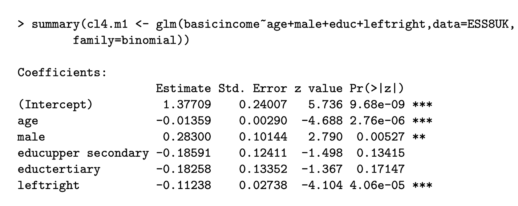
Basic income example: how do you determine the Wald statistic W from this output?

The z-value is \sqrt{W}.

So W=z².

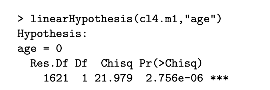
Basic income example: What is this testing? how do you determine the Wald statistic W from this output?

This is testing the null hypothesis H_0: \beta_{age} = 0

The Chisq term is = W = z²

So if you squared the z-value term in the reg. output you’d get the Chisq value.

Here, we can reject the null that there is no effect of age on support for basic income, therefore we should keep it as a covariate in our model.

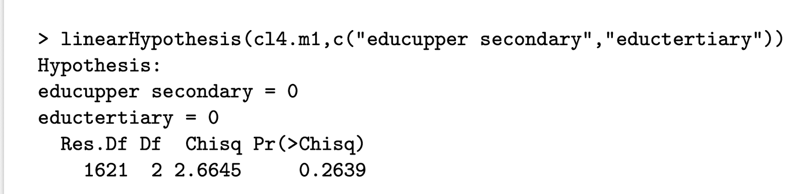
Basic income example: What is this testing?

This is testing the null hypothesis: H_0: \beta_{educ_upper} = 0 AND \beta_{eductertiary} = 0

Finding: the coefficients of the two non-references levels of education are not significantly different from each other, or from zero. Thus education covariate can be removed from the model without loss.

What is the likelihood ratio test (LRT) and when is it used?

The LRT compares nested models, where Model 0 is a restricted version of Model 1

-

It tests whether relaxing constraints (e.g., freeing coefficients) significantly improves model fit

Basic income example: What is the null hypothesis and model comparison for testing whether age matters in the following regression?

glm(basic income ~ age + male + educ + left right, family = binomial)

H_0: \beta_{\text{age}} = 0

-

Model 0: includes male, education, and leftright

-

Model 1: includes these, and also age

Basic income example: What is the null hypothesis and model comparison for testing whether education matters at all? The non-reference categories are educupper and eductertiary

H_0: \beta_{\text{educ upper secondary}} = \beta_{\text{educ tertiary}} = 0

-

Model 0: includes age, male, and leftright

-

Model 1: includes these, and also education as a 3-category variable

Basic income example: What is the null hypothesis and model comparison for testing whether education levels differ from each other?

H_0: \beta_{\text{educ upper secondary}} = \beta_{\text{educ tertiary}}

-

Model 0: includes age, male, leftright, and education as a 2-category variable (grouping upper secondary and tertiary)

-

Model 1: includes these, and education as a 3-category variable

What is the likelihood ratio test (LRT) statistic and its distribution?

G^2 = 2(\ell_1 - \ell_0) compares the log-likelihoods of unrestricted and restricted models

-

Under H_0, it follows \chi^2_{k_1 - k_0} where k_1 - k_0 is the number of constraints tested