BIOL 413 midterm 1

What is a model?

• An abstract description of a concrete system

• Simplified, often mathematical, representation of system

  • Think of daily stimuli

  • “baby speak,” simplified language

Why are models useful and awful?

• simplification of a complex system (main effects)

  • every single model is wrong

Keystone species

High impact animals

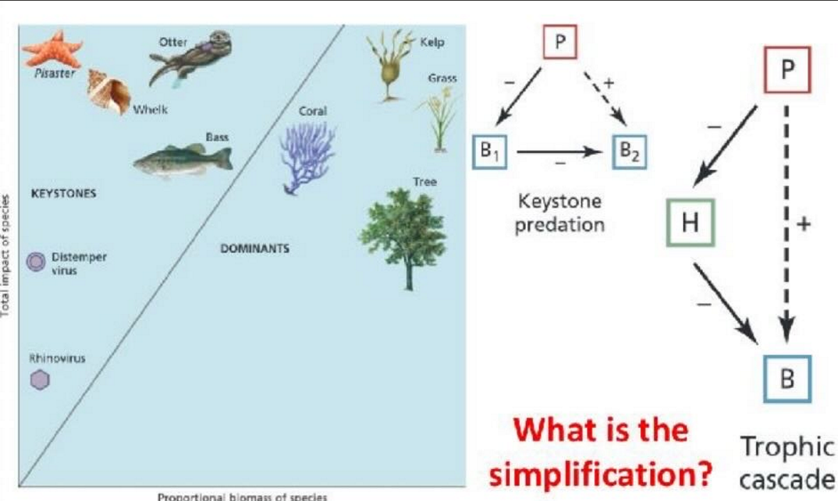
Ecological Modelling

P = predator, H = herbivore, B = basal (animal + plant)

• some models more wrong than others

  • must seek models that are faithful to reality

  • implies a specific purpose

  • a purposeful and faithful simplification of reality

  • models subset of the real world, not the whole world

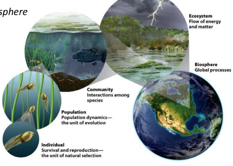
Scales of ecology

Individual→ population→ community→ ecosystem→ biosphere

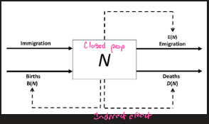
Population

• Individuals of the same species lining in a defined area

  • how are populations described

Studies at population level:

• Emphasis on variation

  • Number

  • Density

  • Composition

Geographic range (distribution/range)

The extent of land or water within which a population lives

Abundance

The total number of individuals

Density

The number of individuals per unit are

Composition (Demographics)

The “makeup” in terms of age, sex or genetics (relatedness)

Community

Collection of all populations living together in a defined area

→ assemblages of species

• boundaries are not always rigid and may cover small or large areas

• Include many types of interactions

  • Predation

  • Competition

  • Herbivory

Studies at community level:

• diversity

  • Richness (Total)

  • Evenness (distribution)

• Species interactions

statements about succession

• Communities follow a pattern of succession at some stable climax of assemblages (wrong statement)—Clements.

  • “super organism”

• Individualistic view: not changes in species assemblages, but responses by individual species to enviromental gradients (more context dependent) - Gleason

  • depends on current enviroment conditions

  • individuals response to individual conditions

Gause's Paramecium experiment

Tested theory on protozoan pop. growing in small bottles, found that species grown separately achieved stable densities but when pairs of species were grown together in a simple environment one species always won out and the other species became extinct

competitive exclusion principle

Two species cannot coexist on one limited resource - Gause

Niche

Range of conditions that a species can tolerate

Fundamental niche

Parts of the environment that a species could occupy in the absence of interactions with other species - abiotic conditions (pre-interactions)

• The range of abiotic conditions

  • range of temperatures

  • Humidity

  • Salinity

Realized niche

the range of biotic and abiotic conditions under which a species can persist (biotic: competition, predation) - post interactive

• the range of abiotic and biotic conditions under which a species can persist

  • determines the geographic

  • large scale

Small scale

variation in the enviroment creates geographic ranges that are composed of small patches of suitable habitat

Reciprocal transplant experiment

When planted outside their natural elevations, the two species grew poorly and experienced lower survival

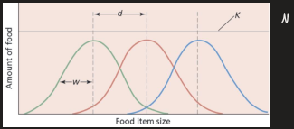
Limiting similarity

Minimal niche difference between two competing species that would allow coexistence

d/w ~ 1

d = separation in mean resources

k = resources continuum

w = standard deviation

• interspecific competition is only primary factor

• universal limits (context dependent)

• greater plurality of factors

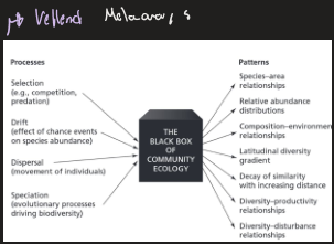
Four factors to explain species diversity

1. Process that determine “success” of species

2. Changes in relative abundance due to chance events

3. Movements of spp in/ out of communities

4. Generation of new species

selection

process that determines the relative success of species w/in a local community

Drift

changes in species relative abundance to chance or other random effects

Dispersal

is the movement of individuals + species into and out of local communities

speciation

operates over spatial scales larger then the local community and it is process that ultimatlt generates diversity in regional species

Patterns of diversity

• patterns of diversity are ubiquitous

  • despite greater area at northern latitudes

  • diversity as species richness larger charismatic organisms

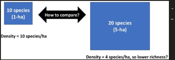
Measuring diversity (species richness)

defining a community boundary is arbitary (quadret, transect)

• problem: richness strongly correlated (+) w/sample size

• richness scales non-linearly w/samples size/affect also arbitary

Type of standirization often works for abundance for biomass, which scales roughly linearly w/area

approach dont work for species richness b/c of non linear relationship between richness + sample size

aspects of diversity

• species richness

• genetic diversity

• functional diversity (how many fitted niches)

• Phylogenetic diversity (how much evolutionary history)

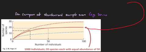
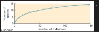
Species accumulation curve

walking through a new community, recording observed species

• green dashed curve is first set of data

• blue curve is multiple random walks which have been averaged

• blue dashed line highly uneven distribution with lots of rare species increasing slowly (encounter common species occasionally encounter rare species)

• if curve is up “increasing deceleration function”

• If curve is down “decreasing deceleration function”

Highly uneven distribution curves with lots of rare species increase slowly

Alpha diversity

The number of species found at a local scale

• richness found at a local scale

Beta diversity

Measure of difference in species composition or species turnover between two or more habitats or local sites within a region

• the change (species turnover) in richness sites w/in a region

Gamma diversity

A measure of species richness in a region

B= a/y

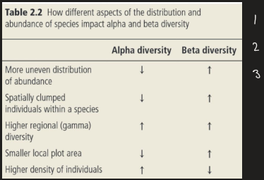
Factors that change alpha & beta diversity

1. Unevenness ( lower a + increased B)

2. Dispersion (clumped vs random) - lower a + increased b

   • similar affect s unevenness

   • Faster increase with random

3. Higher regional (gamma diversity) - decreased a + increased B

4. Smaller local plot area - decreased a + increased b

   • like sampling fewer individuals

5. Lower density of individuals - increase a + decrease B

   • fewer individuals per plot

Species-area relationship (SAR)

S = cA^z

S=number of species

A=area

C&z=fitted constant

• Large areas contain more species than smaller areas

• Larger areas contain greater variety of habitat types

• Different species have different habitat affinities

• Larger areas = more species

  • larger areas support larger populations (lower chance of extinction)

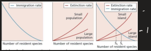
SARs two drivers

• immigration:

  • rate declines with # of resident species (0 when source and sink have the same species)

• Extinction:

  • rate increases with number of resident species

  • Just more species to go extinct

  • Number of individuals/species decreases as total residence increases (smaller populations)

• Even in areas of uniform habitat, larger areas= more species

  • larger areas support larger population (lower chance of extinction)

  • Intersection =equilibrium point (immigration-extinction equilibrium richness

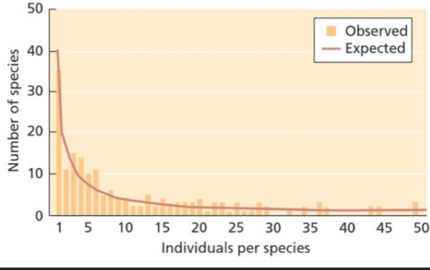
Are most species common or rare?

• most communities:

  • few common species

  • Many rare species

• Many potential causes

  • periodic disturbances (fire, salt marshes)

  • Sampling & transient (migrating) species

    • imperfect

• Competitive exclusion

  • few dominants outcompete

• Freq. dep predation

  • common vs rare

• Genetic variation

  • small = pop low genetic var (vulnerable to disturbance/disease

Productivity and species richness

• broad scales: species richness increases with productivity

  • productivity = conversion of resources to biomass

  • Regional (large scale) positive (sometimes decelerating)

    • high productivity = high richness

• Smaller scale: varies patterns - positive, negative “hump shape”, “U shape”

• productivity peaks at intermediate species richness

  • richness limited by abiotic stress in unproductive environments and a species interaction in productive ones

• Resources

  • Nutrient limitation + light limitation

• Habitat frequency

  • High/low productivity environments rare

  • Varies from low to high annually average intermediate

Latidudinal diversity gradient

pattern of the tropics having far more diversity than polar regions

Null model

Geometric constrains on species ranges

• pattern generating model that is based on randomization of ecological fate or random sampling from a knwon or imagined distribution

• outcome of placing species ranges on a bounded domain - mid domain effect

Criticisms

1. is it truly neutral to processes it claims to rule out (climate)

2. Fitting observed data to model (high variance) applies to mammals + elevation

3. Predicts high diversity in centre of continents (not found)

Ecological hypotheses

Focus on carrying capacity (K) of an area

Ecological hypotheses: climate

Water important to life

Strong climate species richness correlation (especially broad scale)

• more individuals (species-energy) hypothesis

  • richness varies with climate because

  1. Number of individuals that an area can support increases with primary productivity (available energy)

     • greatest in tropics (warm/humid)

  2. Greater species richness in areas that can support more individuals

     • more individuals divided among more species

• Individuals within a group increases with primary productivity

• Number of species increases with number of individuals

• Insufficient to account for species accumulation with decreased latitudes

• Expect more species in smaller populations in warmer climates

why are there more species in the tropics than expected

species individual curve varies across climate regions not constant increase in speces

what if species could persist at smaller population sizes

expect more species in smaller population in warmer climates

Historical explanations

Geological history and available time for diversification

• tropics more diverse b/c of more time

High latitudes: periodic ice ages and glaciation species richness

Low altitudes: more stable and benign

Historical explanation: geological history and the time for diversification (LDG goes back to Cenozoic)

Time integrated area hypothesis:

• combined effects of time and area

• requires low dispersal rates between temperature and tropical regions

Two effects

1. Positive effects of area (more tropics) on speciation rates

2. Decline in extinction rates with area

tropical niche conservatism

• tropical species stay at tropical

• latitudinal diversity gradients strengthen + weaken several times over histort

  • should have been maintained at low latitude

Evolutionary

Higher diversification rates in tropics

Diversification. = specification rate - extinction rate

• population growth rate = births - deaths (closed populations)

higher diversifications rates in tropics due to greater speciation and lower extinction

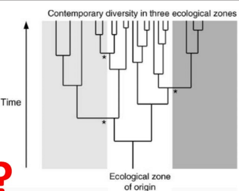
where do more (contemporary) species originate?

• rate = sp events/time

• adaptive shift to different eco. zone = *

speciation rates at tips of tree

• >= in temperate zone relative to tropics

speciation rates integrating recent + past

• > speciation

Probability of speciation + extent of division increases closer to equator

More endemic fish near equator

• more opportunities for geo isolation (reproductive barriers)

• Higher mutations rare & shorter generation in tropics

• Stronger species interactions

Endemism

Indicates at least one speciation event at each site

Number of endemics

Estimate of extent of diversification (sp-ex)

Ecosystem functioning

• productivity (primary

  • nutrient cycling & retention

  • how many species required to move mass of elements

  • atmosphere - hydrosphere - litho sphere

• Disturbance resilience & stability

  • community recovery after disturbance

• Ecosystem multifunctionality

  • are all species equally effective in functioning

  • how mant functions by each species

Diversity & productivity

higher species diversity leads to higher ecosystem producticity

three studies:

• Cedar creek ecosystem science reserve

• BIODEPTH

• Jena biodiversity experiment

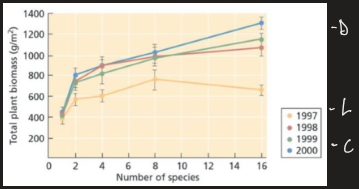
Cedar creek

• plots w/1,2,4,8,16 grassland savannah

• productivity nutrient dynamycs, stability for 20 yrs

• productivity measured as biomaa

• drastic increase in adding few species

  • becomes asymptotic w/more

• lower productivity in 1997

• criticism/limitation

  • only 1 single location

  • same species in all plots

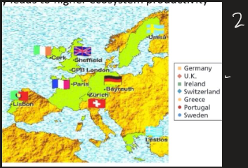
BIODEPTH (Biodiversity + ecological proccesed in terrestrial herbaceous ecosystems

• similar design to cedar creek 

  • replicated in 7 countries

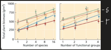
jena biodiversity experiment

• manipulated plant diversity:above/below biomass & nutrient use

• unique:richness & functional groups (types of species)

findings of all studies

• pos. deceleration relationship

• suggests some species can be lost before collapse of productivity

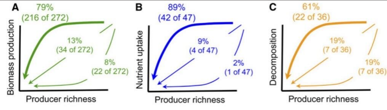
Corinale meta analysis

• 368 experiments

  • terrestrial, fresh water, marine

  • plant types

→ generalize to primary producers

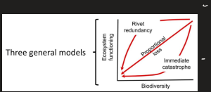
proportional loss: linear relationship

• 1 change in biodiversity = 1 change in ecosystem function

Rivet redundancy: redundancy of species so if 1 goes extinct, ecosystem doesnt collapse b/c on rebundant species that does the same

• multipple species that fill role of multiple functional groups

immediate catastrophe: even a small decrease in biodiversity results in decrease in ecosystem

• saturating function (michaelis manten curve)

• productivity: 79% (pos. & decelerating)

3 aspects

A. primary productivity

B. Nutrient uptake → how effecient communities are utilizing resources

C.Decomposition → Nutrient cycling, returning nutrient back to soil

Caution in a strict + literal interpretation

1. one aspect of diversity (richness)

2. relative importance of large early vs small later change in richness under field conditions & tipping point

→ study counting all species as equal not realistic

Assumption “saturated model”

• function can be extrapolated to estimate max. biomass production as species richness goes to infinity

→ literal interpretention not advised

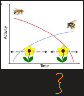
niche complementarity (resource partitioning)

• when species differ in how they use a limiting resource

  • differ in phenology, physiology, nutrient requirements

• species niches differ

• increases resource use efficiency

• more species (increased species richness)

  • increased productivity

    • from “facilitation”: N-ficing & non fixing species

species selection (sampling effects)

• increasing productivity if diverse communities are dominated by few highly productive species (uneven communities)

operate in concert

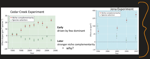
species selection early - niche complementarity later

• detected through Transgressive overyeilding- mixed plots yield more biomass (compared to any monoculture) increases w/community maturation

• species selection effects may be dominant drivers of ecosystem functioning  early in on experiment

• niche complementarity effects becomes stronger as communities mature

• Niche complemantarity increased over time, while species selection effects decreased over time (cedor)

• effects of species richness on ecosystem functioning become stronger over time (jena)

→ temporal strengthening of biodiversity due to combo of increased ecosystem functioning at low biodiversity

if species empty niche complementary (resource partioning)

1. diverse communities more efficiently use resources

2. amount of unused resources decline w/more species (richness)

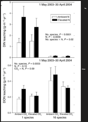
Nitrogen and leaching

• reduced available N concentration in soil

  • increase in plant species richness reduces available N concentration in soil

• increase in N in (above ground) biomass w/higher diversity

  • efficiency of nutrient uptake

• correlated positively w/species diversity indicating total N uptake increased w/increasing diversity

• less DIN (dissolved inorganic N) leaching

  • more efficient uptake by plant community

  • increasing in plant richness reduced leaching loss of DIN as consequence of more efficient nutrient uptake by plant community

  • DON does not dissolve easily + may not be directly available for plant uptake

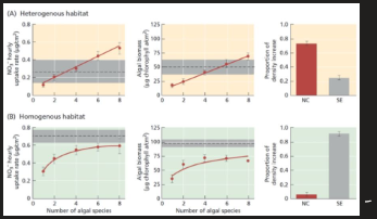
Heterogenous vs homogenous

A: heterogenous (niches) streams

B:homogenous (no niches) stream

= highest rate/biomass of 1 species in monocultue

• nitrogen run off into streams + rivers, significant source of pollution

  • in labs w/high heterogenesity an increased in algal species richness, reduced amount of DON in stream water

  • more homogenous, loss of opportunities for drift algal species led to reduced algal diversity + reduction in N uptake

  • pos. effects of algal species richness on water quality due to niche complementarily

Measures to stability

• species richness

• Species evenness

• Productivity

• Interactions (abiotic/biotic)

• Rate (change) of growth

• Amount of habitat suitability

• Diversification rate

• Time to base state

→ common theme: time

Dynamical systems

Systems that change over time

• alternative stable states

• Non point attractors

• Extinctions

• Invasion

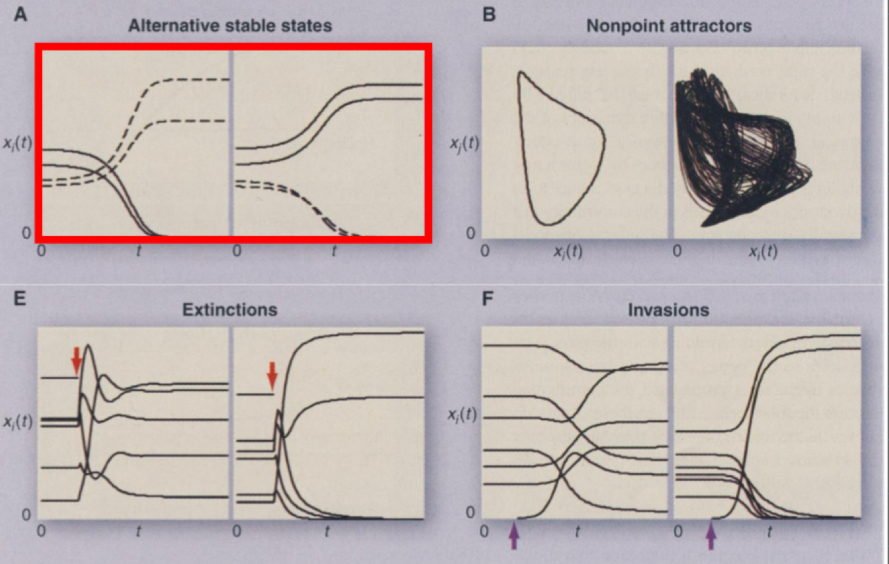
Alternative stable states

• initial (density) conditions

  • determines persistence

    → population abundance initial condition determine how they end up

• Initial conditions determine outcome

• Stability

  • # of stable states

    • few = more stable

      → the more alternatives the less stable; vice versa

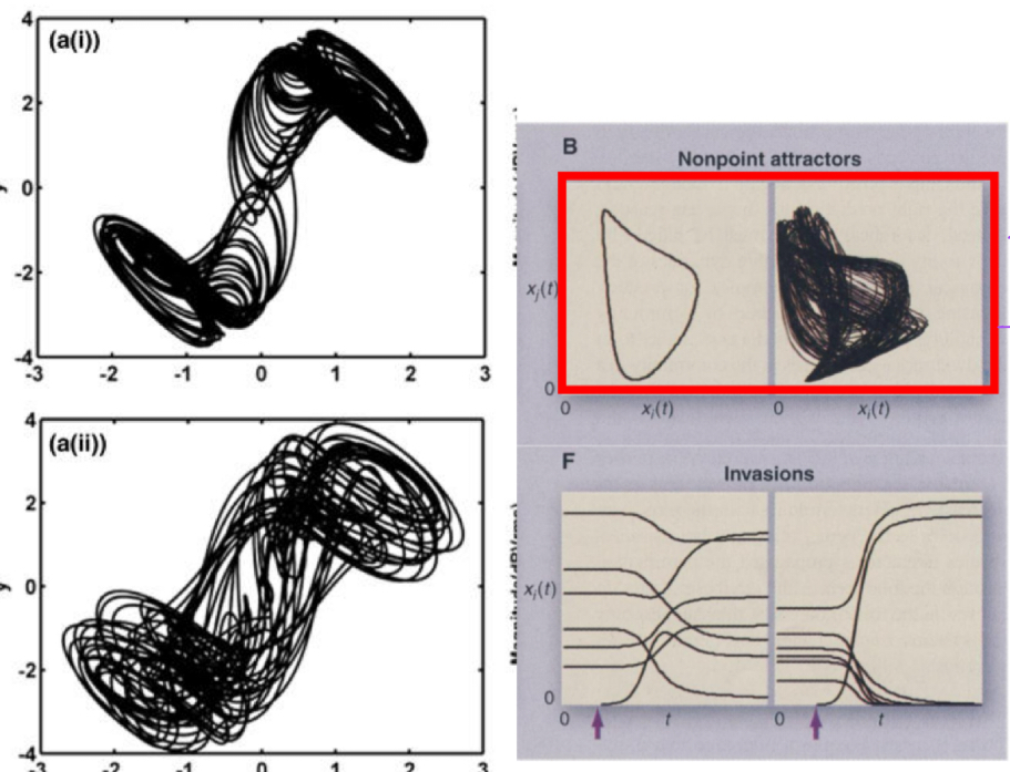
Non point attractors

• no point equilibrium (pre-prey)

  • perpetual density oscillations

• Stability

  • low vs high chaos

• Change in predator over time

  • increase w/pret abundance, decrease w/lack of prey

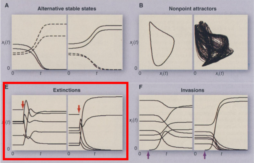
Extinction

• stability

  • how many other species go extinct

    • fewer = more stable

• Density of surviving species

  • little changes = more stable

    • Little alternatives = more stable

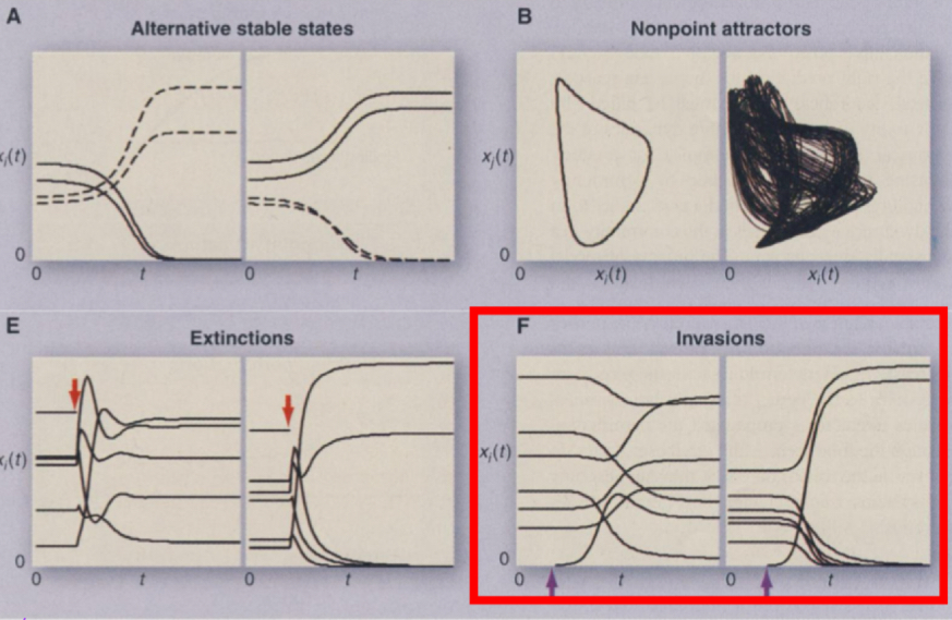
Invasions

• Stability

  • chance of successful invasion

    • Low = more stable

  • # of secondary extinction

    • few = more stable

      → more species go extinct w/succesful invasion more extinction = less stable

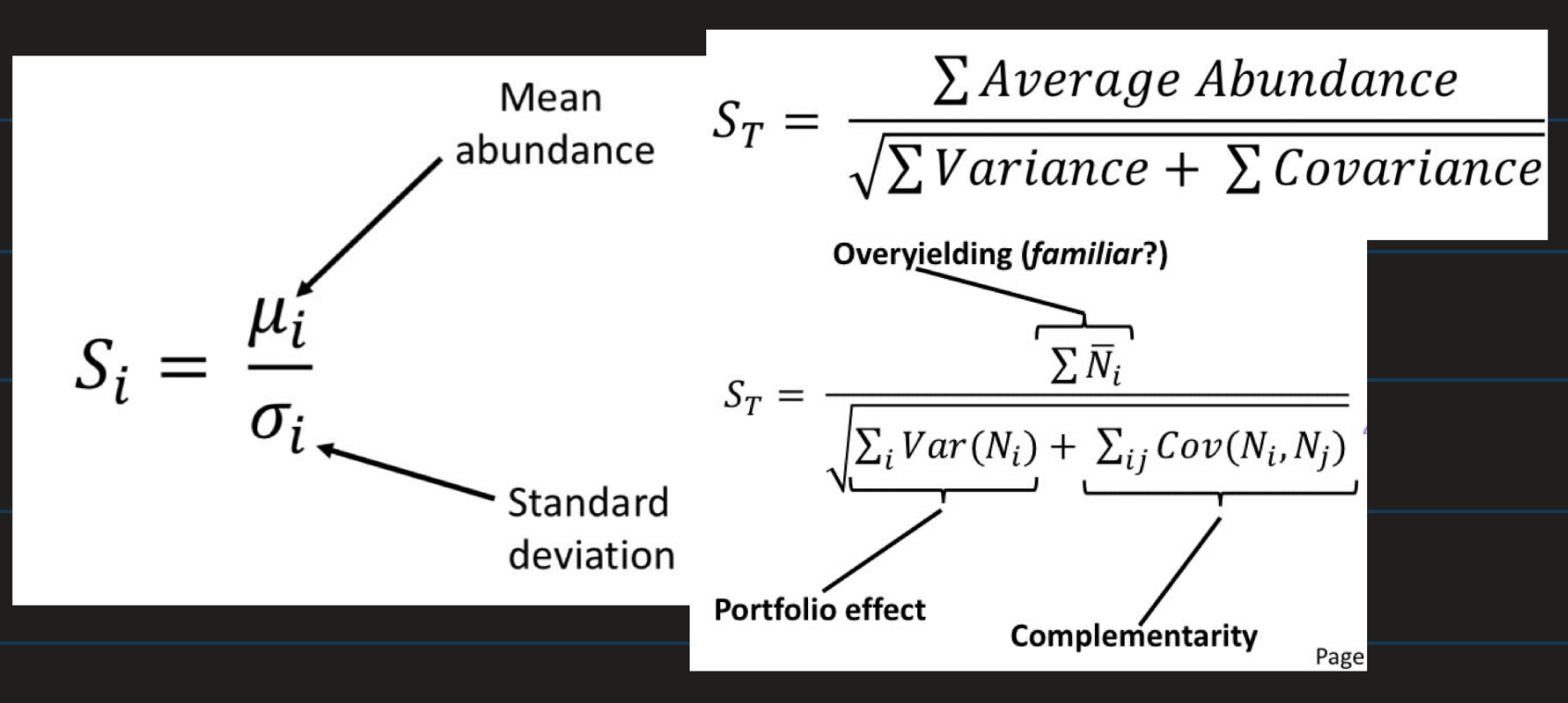
Temporal stability

Focus:

• consistency of a quality over time

  • (abundance of species)

Stability:

• variance in species abundance, overtime + scaled to mean abundance

Applied to:

Specific species

Entire community

Overall species

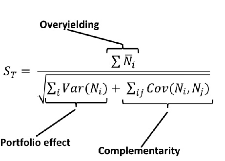
Community stability

Diversity (richness) increases St when

Increase Ni

• Total sp abundance

Decreasing Var, Ni

• Summed var

Decreasing Cov(Ni,No)

• summed covariant

Increase (total sp abundance)

• increase species richness

  • you are increasing community productivity

• Over yielding increasing temporal stability

What if diversity does not affect total community biomass

• species fluctuate randomly/independently cov (Ni,No)=0 + reduces var(N)

• Increase richness reduces summed variance - portfolio effect

Correlated responses to environment

• any negactive covariance will increase St

• Any positive covariance will decrease St

Types of interactions

• negative coviarence (Ni,Nj)

  • interspecific competition

    • positive effect on stability

• Positive covariance (Ni, Nj)

  • Facilitative mutualism

    • negative effect on stability

Foundational species

• creates/engineers physical structure of ecosystems - form base of community

• General abundant/dominant species

• Often near the base of food webs

Ecosystem engineers

• Not a base

• Not a abundant/dominant

Beavers (Dam/lodge flooding)

• water quality (filter)

• Flood/drought mitigation

• Fire management (water & cutlines)

• Biodiversity (at least 50% threatened species)

Trees (forest)

• habitat

• Food

• Soil conditions

Coral (coral reef)

• shelter

• Habitat

Ecosystem function

• nutrient cycling

• Decomposition rates

• Energy flow

• Carbon capture

• Chemical cue transmission

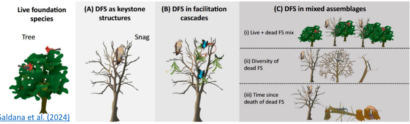
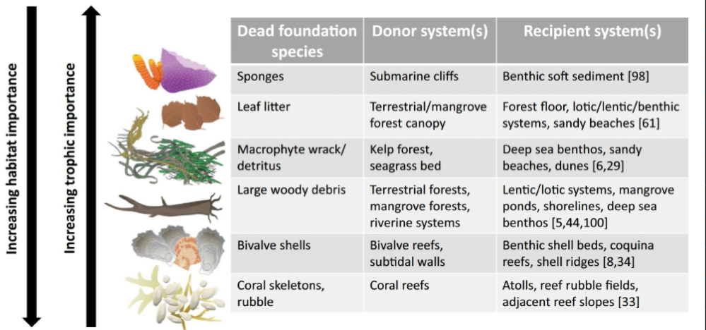
Dead foundational species: habitat heterogeneity

Keystone structure

• unique structure providing resource (insects- consumers, birds habitat) (different from living foundational species effect)

Facilitation cascade

• primary species facilitates secondary species facilitates others species, dead tree, secondary epiphytes insects other bird consumers (hierarchical)

Mix of living (foundational effects) and dead, species mix (different effects) time since death