Booklet 8 - The Aggregate Expenditure Model

List the Factors Affecting Each of the Components of Aggregate Expenditure

Aggregate Expenditure (AE)

Gross Domestic Product (GDP)

Define Aggregate Expenditure (AE) & Provide the Formula

The sum of all expenditure on final goods and services undertaken in the economy during a specific time period

AE = C + Ip (planned investment) + G (G1 & G2) + (X-M)

Define Gross Domestic Product & Provide the Formula

The final value of all goods and services produced in a country during a year.

GDP = C + Ia (Actual Investment) + G + (X-M)

Differentiate between AE & GDP

The difference between AE and GDP is that the value of inventories (unsold stock) is included as part of the actual investment when calculating GDP whereas it is not included in planned investment when calculating AE.

What do you Discuss when Asked about the - Categories of Consumption:

Identify the Proportion of AE Consumption Accounts for

1. Expenditure on Non-Durable Goods

2. Expenditure on Durable Goods

3. Expenditure on Services

What Proportion of AE does Consumption Account for

52%

What are the Categories of Consumption:

1. Expenditure on Non-Durable Goods
   Expenditure on non-durable goods refers to spending on items that are consumed quickly, typically within three years, such as food, beverages, packaged products, clothing, and footwear. Much of this spending is essential or non-discretionary, satisfying regular household needs, and is relatively stable over time, typically accounting for around 35% of total consumption expenditure.

2. Expenditure on Durable Goods
   Expenditure on durable goods involves spending on items that last three or more years, such as major appliances (fridges, washing machines), small appliances (kettles, toasters), sporting equipment, and motor vehicles. This type of spending is generally discretionary, meaning it can be postponed or brought forward depending on a household’s financial situation. Durable goods account for roughly 15% of total consumption expenditure.

3. Expenditure on Services
   Expenditure on services refers to spending on intangible goods that provide transitory satisfaction, including education, transport, health, and recreation. Services make up the largest portion of household consumption, accounting for around 50% of total expenditure. Some services are essential, such as health and transport, while others, like entertainment and leisure, are discretionary.

What do you Discuss when Asked About - the Factors Affecting Consumption

Level of Disposable Income (Yd)

Interest Rates (Cost of Credit)

Government Policy

Consumer Expectations

Asset Prices (Household Wealth)

Other Demographics)

Discuss Level of Disposable Income (Yd) as a Factor Affecting Consumption

The level of disposable income (Yd) is a key determinant of consumption, as it represents the income households have available after tax. There is a positive relationship between disposable income and spending—when households’ disposable income rises, consumption increases, boosting aggregate expenditure. For example, during a boom, higher incomes encourage greater household spending.

Succinctly Discuss Interest Rates (Cost of Credit) as a Factor Affecting Consumption

Interest rates, as the cost of borrowing and return on saving, directly affect household consumption. Low interest rates reduce the cost of servicing debt and lower the opportunity cost of spending, encouraging greater consumption and boosting aggregate expenditure. Conversely, high interest rates increase borrowing costs and make saving more attractive, reducing household consumption and aggregate expenditure.

Succinctly Discuss Government Policies as a Factor Affecting Consumption

Government policies influence household consumption through both monetary and fiscal measures. Contractionary monetary policy, such as increasing the cash rate, raises borrowing costs and reduces household spending power, lowering consumption. Similarly, contractionary fiscal policy, through higher taxes or reduced government spending, decreases disposable income and aggregate consumption. Both policies serve to moderate spending and aggregate expenditure in the economy.

Succinctly Discuss Consumer Expectations as a Factor Affecting Consumption

Consumer expectations influence spending decisions based on positive or negative sentiments about the economy. Optimistic expectations, driven by factors like economic growth, interest rate changes, and asset market trends, encourage households to increase consumption, thereby raising aggregate expenditure

Discuss Asset Prices (Household Wealth) as a Factor Affecting Consumption

Household wealth, the difference between assets and liabilities, influences consumption. When asset values such as property, shares, or savings rise, households feel wealthier and more confident, leading to higher consumption and increased aggregate expenditure in the economy.

Discuss Asset Prices (Household Wealth) as a Factor Affecting Consumption

An increase in population, increases consumption on goods and services and this will increase aggregate expenditure in the economy. Example: Australian economy

What do you Discuss when Asked About - Categories of Investment

Identify the Proportion of AE accounted for by Investment

Business Investment

Housing Investment

Proportion of AE accounted for by Investment

19%

Composition of Investment Spending

Business Investment

Privately funded business spending on capital goods used in production. This includes equipment, machinery and buildings.

Housing Investment

Private expenditure on new housing and apartments.

What do you Discuss when Asked bout Factors Affecting Investment

Interest Rates (Cost of Credit)

Level of Past Profits

Business Expectations

Government Policy

Discuss Interest Rates (Cost of Credit) as a Factor Affecting Investment

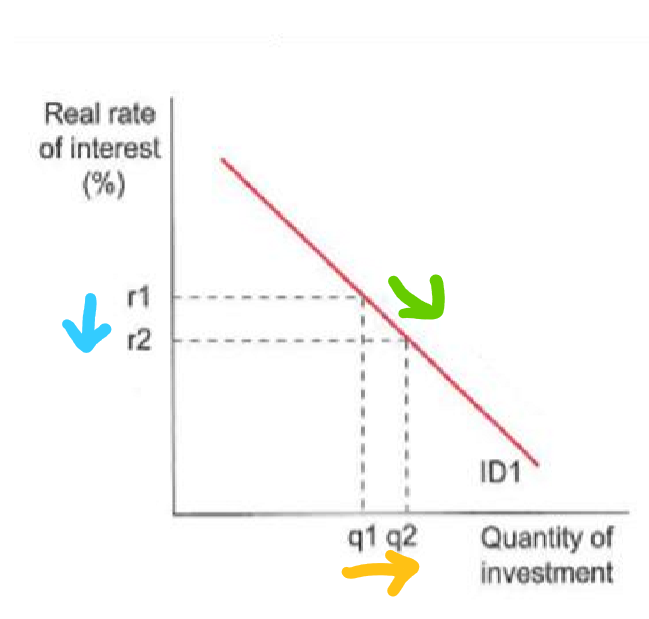
The rate of interest plays a key role in business investment decisions. Interest rates and the level of investment expenditure are negatively related. This concept is illustrated in the investment demand curve below.

Higher rates of interest (r1) tend to reduce investment expenditure (q1). If interest rates decrease from r1 to r2, there would be a movement down the investment demand curve (ID1), and investment would expand from point q1 to q2. This would increase investment expenditure and therefore aggregate expenditure.

Nominal interest rates are the current price of borrowed money whereas the real interest rate takes into account inflation. Real interest rates are more important to decision makers because they reflect the true cost of borrowed money.

Discuss Level of Past Profits as a Factor Affecting Investment

The level of past profits affects investment expenditure by determining the funds firms have available for expansion. When profits are high, firms can invest in new capital, equipment, or premises, increasing aggregate expenditure. Conversely, low profits during economic downturns limit available funds, reducing investment and aggregate expenditure.

Discuss Business Expenditure as a Factor Affecting Investment

Business expectations influence investment expenditure by shaping firms’ confidence in future sales and profits. Positive expectations encourage firms to increase planned investment, boosting aggregate expenditure, while negative expectations reduce planned investment, lowering aggregate expenditure.

Discuss Government Policies as a Factor Affecting Investment

Government policies affect private investment through both monetary and fiscal measures. Contractionary monetary policy, such as higher interest rates by the RBA, increases borrowing costs for businesses, reducing investment expenditure. Similarly, contractionary fiscal policy, like higher company taxes or a budget surplus, lowers available profits for firms, decreasing investment and aggregate expenditure.

What do you Discuss when Asked about - Categories of Government Spending

Identify the Proportion of AE Government Spending Accounts for

Current spending

Capital Spending

Identify the Proportion of AE Government Spending Accounts for

29%

Categories of Government Spending

Current Spending

Expenditure on the day-to-day business of government in its core functions like health, education, social welfare and defence. This includes wages and salaries and the purchasing of goods and services.

Capital Spending

Spending on productive machinery and public infrastructure such as power and water supply, roads, railways and communication networks. Government spending has a cyclical and structural element to both G1 and G2. These will be examined in more detail in the Fiscal Policy booklet.

What do you Discuss when Asked About - the Factors Affecting Government Spending

Discretionary Changes (Optional Changes)

Automatic Changes (Forced Changes)

Stabilising Macroeconomic Fluctuations (Economic Obligations)

Discuss Discretionary Changes (Optional Changes) as a Factor Affecting Government Spending

Governments will increase and decrease spending in accordance with government policy objectives such as social policies, infrastructure, health and education. For example, the Federal Government is contributing $1.7b to Perth’s Metronet project (G2). This increases government spending and therefore increases aggregate expenditure.

Discuss Automatic Changes (Forced Changes) as a Factor Affecting Government Spending

Automatic changes in spending will occur depending on the phase of the business cycle. In a contractionary phase, there will be more unemployment and therefore government spending on welfare will increase. For example, during the Covid pandemic, government spending on welfare payments such as JobSeeker (G1) increased therefore increasing aggregate expenditure

Discuss Stabilising Macroeconomic Fluctuations (Economic Obligations) as a Factor Affecting Government Spending

In a contractionary phase, governments may actively increase spending in an attempt to increase economic activity. For example, during the pandemic, increases in Jobkeeper (subsidy) and Jobseeker (transfer payment), caused government spending (G1) to increase therefore increasing aggregate expenditure

What do you Discuss when Asked About the Categories of Net Exports (X-M)

Identify the Proportion of AE Accounted for by Net Exports

Imports

Exports

Identify the Proportion of AE Accounted for by Net Exports

3%

Categories of Net Exports (X-M)

Imports

Foreign purchases of goods and services produced in Australia are exports and add to aggregate expenditure.

Exports

Imports occur when Australians purchase goods and services from overseas and reduce aggregate expenditure.

What do you Discuss when Asked About - Factors Affecting Net Exports

Level of Economic Activity

Exchange Rates

Terms of Trade

Presence of Trade Barriers

Discuss Level of Economic Activity (Domestic Economic Activity & Overseas Economic Activity) as a Factor Affecting Net Exports

Domestic and overseas levels of economic activity directly affect Australia’s net exports. Domestically, higher economic activity increases households’ and firms’ demand for imported goods and capital equipment, reducing net exports and aggregate expenditure. Conversely, stronger economic activity overseas raises income and employment in other countries, increasing their demand for Australian exports, which boosts net exports and aggregate expenditure.

Discuss Exchange Rates as a Factor Affecting Net Exports

An appreciation of the Australian dollar increases Australians’ purchasing power, making imports cheaper and raising import levels, while simultaneously reducing the international competitiveness of Australian exports (excluding commodities). Both effects decrease net exports and, consequently, aggregate expenditure.

Succinctly Discuss Terms of Trade as a Factor Affecting Net Exports

An improvement in the terms of trade, reflected by an increase in the export price index (XPI) relative to the import price index (MPI), raises exporters’ income and the value of exports. Simultaneously, lower import prices reduce the value of imports, boosting net exports and increasing aggregate expenditure.

Succinctly Discuss Presence of Trade Barriers as a Factor Affecting Net Exports

Trade protection, such as tariffs or quotas imposed by Australia’s trading partners, can reduce the demand for Australian exports. This decreases exports, lowers net exports, and ultimately reduces aggregate expenditure.

What do you Discuss when Asked About - The Relationship Between the Consumption Function, the Marginal Propensity to Consume and the Marginal Propensity to Save

Average Propensity to Consume Definition & Formula

Average Propensity to Save Definition & Formula

Formula for the Average Propensity to Consume

The proportion of total income that is spent on consumption

APC = Consumption (C) / Income Y

Formula for the Average Propensity to Save

The proportion of total income that is saved

APS = Savings (S) / Income (Y)

What do You Discuss when Asked About - The Consumption Function

Explanation of Autonomous Consumption

Explanation of & Formula for Induced Consumption/Marginal Propensity to Consume

Explanation of Autonomous Consumption

The part of consumption which occurs even when income is zero. This is the minimum quantity of goods to survive. It is constant and does not vary with income. It is the vertical intercept- the point where the consumption function meets the y-axis

Formula for Induced Consumption/Marginal Propensity to Consume

The part of consumption which occurs because income increases. Another name for b is the Marginal Propensity to Consume (MPC). MPC is the fraction of an increase in income spent on consumption.

MPC = Change in Consumption / Change in Income

Formula for the Savings Function

S = d (dis-savings) + e(marginal propensity to save)Y(income)

What do you Discuss when Asked About the Savings Function

Formula

Explanation of Dis-Savings

Explanation of & Formula for Marginal Propensity to Save (MPS)

Explanation of Breakeven Point

Formula for the Savings Function

S = d (dis-savings) + e(marginal propensity to save)Y(income)

Explanation of Dis-Savings

The minimum level of dis-savings in the economy. When savings is negative, this is defined as dis-savings. This is due to the autonomous consumption in the macroeconomy. Every person must consume a minimum quantity of goods to survive even if income is zero (i.e., food, shelter, clothing etc). It is the use of past-savings when income is less than spending.

Explanation of & Formula for Marginal Propensity to Save (MPS)

MPS is the fraction of income that is not spent on consumption. MPS is the slope of the savings function.

MPS = Chane in Savings /Change in Income

What do you Discuss when Asked About the Aggregate Expenditure (AE Model)

Define Consumption

Define Investment

Define Government Spending

Define Exports

Define Imports

Define Consumption in reference to AE (Full Keynesian AE Function)

Has both an autonomous level and an induced component. The autonomous level is the minimum amount of consumption necessary for economic participants to survive, while induced consumption depends on income (GDP) and is determined by the marginal propensity to consume (MPC).

Define Investment in reference to AE (Full Keynesian AE Function)

Assumed to be independent of income and thus considered autonomous. This assumes that factors affecting investment, such as interest rates and expectations, remain constant.

Define Government Spending (G) in reference to AE (Full Keynesian AE Function)

Independent of the level of GDP and is therefore considered autonomous. This assumes that factors affecting both discretionary and automatic spending are constant

Define Exports (X) in reference to AE (Full Keynesian AE Function)

Independent of the level of income and thus autonomous

Define Imports (M) in reference to AE (Full Keynesian AE Function)

Similar to consumption. There is an autonomous level of imports and an induced component that depends on income (GDP). Induced imports increase with real GDP.

Assumptions of the Consumption Function & Savings Function

MPC + MPS = 1. MPC and MPS do not vary with income – they are established independently and will be constant. APC and APS do change with incomes as they’re dependent on income.

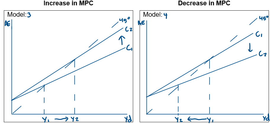
A change in income will cause a movement along the consumption function while a change in non-income determinants of consumption (wealth, expectations, credit, taxes) will cause a shift of the line upwards or downwards.

If a consumption function is steeper, it means that households spend a greater proportion of any increase in income (Y) they receive. The higher the value of the MPC, the steeper the consumption curve

The Concept of Macroeconomic Equilibrium, Including the Role of Inventories

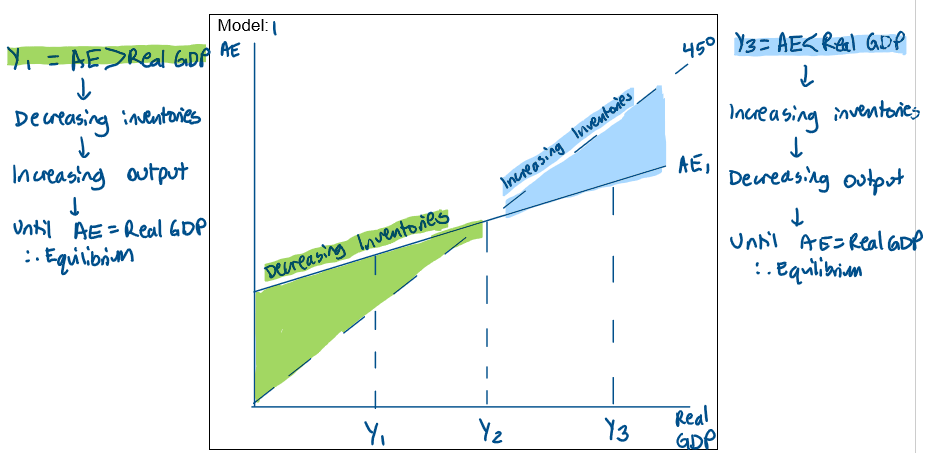
At Y₁, AE is greater than real GDP, leading to a decrease in inventories as firms sell more than they produce.
The reduction in inventory levels signals firms to increase their production to meet the higher demand.
To boost production, firms will hire more labour thereby increasing employment.
This increase in production & employment leads to a rise in real GDP.
However, as real GDP rises the increase in AE slows due to the slope of the AE curve which reflects the MPC.
The economy continues to adjust until it reaches a new macroeconomic equilibrium at Y₂ where AE equals real GDP & income levels are stable.
At Y₃ real GDP exceeds AE resulting in increasing inventories as firms produce more than what is being consumed.
The accumulation of inventories signals firms to decrease their production to prevent excess unsold goods.
As firms reduce production, they demand less labour leading to a decrease in employment.
This reduction in production & employment causes a decline in real GDP.
As real GDP falls the decrease in AE occurs at a reduced pace due to the slope of the AE curve which moderates decline & reflects the MPC.
The economy adjusts until it reaches a new macroeconomic equilibrium at Y₂ where AE equals real GDP & income levels are stable.

What do You Discuss when Asked About - The Concept of the Multiplier

Define Multiplier

Define Positive Multiplier

Define Negative Multiplier

Multiplier Formula (k)

Change in Income Formula 

Characteristics of the Multiplier

Size of the Multiplier

Complex Multiplier

Tax Multiplier

Define Multiplier

A coefficient (or number) which relates to a given change in investment to a final change in the level of income.

Define Positive Multiplier

Whereby an increase in autonomous spending creates a larger increase in income

Define Negative Multiplier

Whereby a decrease in autonomous spending creates a larger decrease in income.

Multiplier Formula (k)

K = 1 / MPS

or

K = 1 / (1-MPC)

Change in Income Formula 

Change in Y = K x Change in Autonomous Spending

Characteristics of the Multiplier

• The multiplier takes time to work.

• The effect is not immediate.

• The rounds of spending and spending take months or years. • The multiplier works in both directions.

• A rise in the level of autonomous investment results in an even larger increase in the level of income.
  Example:
  Construction of Melbourne’s North East Link (highway/road network) estimated at $26.1 billion ($3.3 billion by the Federal Government in 2024/25)

• A reduction in the level of autonomous investment means a larger decrease in the level of income (the multiplier in reverse).
  Example:
  Covid 19 recession, large decrease in investment due to uncertainty.

• The size of the MPC and the multiplier are directly related. The higher the MPC, the higher the value of the multiplier.

Size of the Multiplier

The size of the multiplier depends on the economy’s marginal propensity to consume (MPC). A higher MPC means more of each additional dollar is spent, resulting in a larger multiplier and a steeper aggregate expenditure (AE) curve. Conversely, a higher marginal propensity to save (MPS) reduces spending, producing a smaller multiplier and a flatter AE curve.

Discuss the Complex Multiplier

Define Complex Multiplier

Any change in the components of the AE will give rise to the multiplier effect. Hence a change in Consumption, Government Spending, Investment and/or Net Exports can trigger the multiplier. A complex multiplier takes all leakages and injections into account and would have this formula:

Complex Multiplier Formula:

K = 1 / (MPS + MPT = MPM)

or

K = 1 / (1-(MP Spend)

MPS: Marginal Propensity to Save

MPT: Marginal Propensity to Tax

MPM: Marginal Propensity to Import

K: Multiplier

What do you Discuss when Asked About the Tax Multiplier

Define the Tax Multiplier

Formula for the Tax Multiplier

Explanation of the Paradox of Thrift

Define the Tax Multiplier

A concept in economics that shows how changes in taxes affect the overall economy. Specifically, it measures the impact of a change in taxes on the total output or income (GDP) of an economy.

Formula for the Tax Multiplier

Ktax = MPC / (1-MPC)

Explanation of the Paradox of Thrift

While saving is a good thing for the individual household, it may not be a good thing for the economy as a whole. Savings benefits the individual but too much saving may lead to a fall in the level of income, output and employment.

Savings depends on income and falling income levels means that households will actually fail in their attempt to save more.

This is known as the paradox of thrif

The multiplier shows how an increase in planned injections into the economy leads to a larger increase in output and income.
This is because the initial injection sets off rounds of spending. It is based on the idea that ‘one man’s spending is another man’s income’.
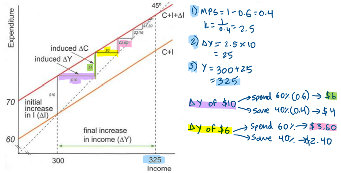
In the first round investment, a new income of $10b is generated for workers to either spend or save their income.
Assume in a mining venture, workers such as engineers and construction workers are employed and paid for their labour.
As MPC is 0.6, workers spend $6b on goods and services and save $4b.
In the second round, as $6b is spent by the first group of people.
This will flow into other groups of the economy and they will receive $6b as their income.
Assume the workers in the mining site venture out to buy food from Woolworths.
The employees at Woolworths will receive a new income of $6b.
These second group of employees will spend 60% of $6b (which is their new income) and save 40%.
Remember MPC is 0.6 and MPS is 0.4.
As a result the new income generated of $6b allows employees to spend $3.6b and save $2.4b.
In the third round, a new income of $3.6b has been created.
Woolworths employees are able to receive a new income of $3.6b and they will spend 60% ($2.16b) & save 40% ($1.44b).
This cycle of one man’s spending is another man’s income continues a new level of equilibrium has been reached and when income is equal to zero.
Any initial change in spending will set of a chain reaction of spending and re-spending which leads to a magnified increase in the level of income.
This is known as the multiplier process.

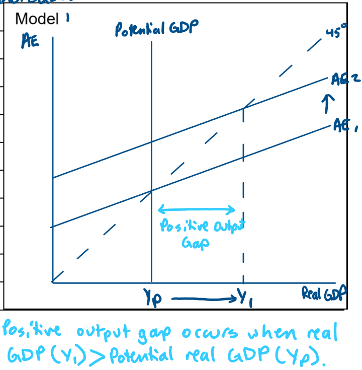
Positive Output Gap

The economy is in an equilibrium at potential GDP (Yp).
An increase in autonomous AE shifts the aggregate expenditure curve upwards from AE1 to AE2.
This causes a positive multiplier effect whereby the increase in autonomous AE from AE1 to AE2 creates a larger increase in real GDP from Yp to Y1.
This creates a positive output gap where actual real GDP (Y1) is larger than potential real GDP (Yp).
At this point the unemployment rate will have fallen below the natural rate & the inflation rate will likely increase.

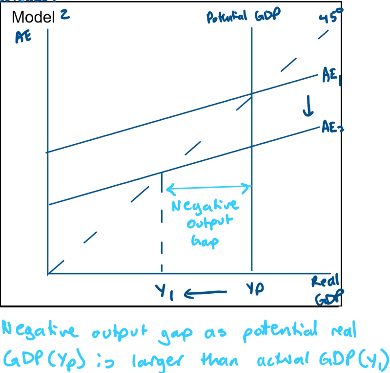
Negative Output Gap

The economy is in an equilibrium at potential GDP (Yp).
An decrease in autonomous AE shifts the aggregate expenditure curve downwards from AE1 to AE2.
This causes a negative multiplier effect whereby the decrease in autonomous AE from AE1 to AE2 creates a larger decrease in real GDP from Yp to Y1.
This creates a negative output gap where actual real GDP (Y1) is smaller than potential real GDP (Yp).
At this point the unemployment rate will have increased above the natural rate & the inflation rate will likely decrease.

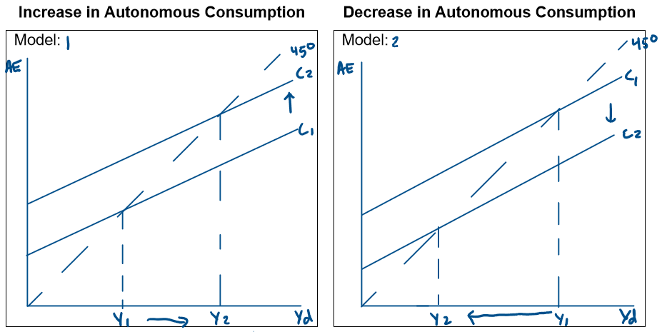
Changes in Autonomous Consumption

The consumption function will shift if any factor that affects autonomous consumption changes. This means that any factor other than income changes. This includes changes in asset prices (wealth effect), consumer confidence etc. This will cause either an increase in consumption which will shift the consumption function upwards or a decrease in consumption which will shift the consumption function downwards.

Changes in the Marginal Propensity to Consume (MPC)

The MPC is the slope of the consumption function, this means that if the MPC increases the slope of the consumption function and therefore the aggregate expenditure function increases, it will become steeper.