PUBPOL 330 - Final Exam Flash Cards

Asymmetric information

When one party possesses information others do not

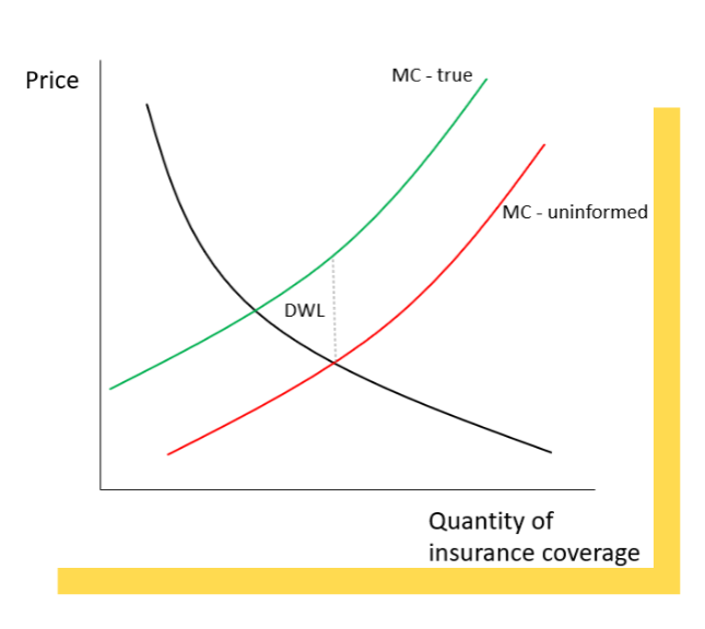
Adverse selection (1)

Sellers have information buyers do not (ie: used car salesman)
● Some insurance buyers try to convince

sellers that MC is lower than it really is

● Another example: labor markets -

employers may know more about

hazardous working conditions than

workers

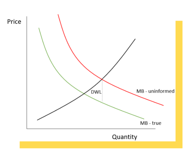
Adverse selection (2)

Buyers have information sellers do not (ie: insurance)
● Sellers try to convince buyers that MB is

higher than it really is

● Examples:

○ The new iPhone 15 is totally different and so

much better!

○ Corporate executives try to convince boards

that hiring them will improve profitability

Moral hazard

You make different choices when your actions aren’t fully observable so you don’t fully face the consequences

When consumers have insurance, they don’t face the full price of their actions, so they tend to be overly risky or over consume (health insurance = using more medical care than would otherwise; disability insurance = riskier than you would be otherwise)

Moral hazard creates the central trade-off of insurance

○ Insurance is desirable for consumption smoothing but creates moral hazard

○ Increases the costs of providing insurance

• Can create reduced precaution against entering the adverse state (auto insurance), increase odds of staying in the adverse state (unemployment insurance), increased expenditures when in the adverse state (health insurance)

Risk

A function of probabilities and payoffs — probability of each outcome and the payoff you’ll receive if each outcome occurs

Fair bet

A gamble on average / in expectation that will leave you with the same amount of money

Risk adverse

Dislikes risk and avoids fair bets; reflects the pain of a loss exceeding the gain from an equal-sized win; arises from diminishing marginal utility; positive risk premium, U is √x

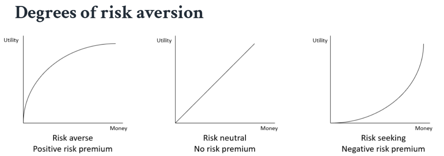
Risk neutral

No risk premium; cares only about expected value of money; risk is irrelevant (risk premium = 0), U is x

Risk seeking

Negative risk premium; gains utility from taking risks, U is x²

Expected value

Average payoff from a risky choice
Probability-weighted average of payoffs associated with all possible outcomes

= Probability(outcome 1) * Payoff(outcome 1)

+ Probability(outcome 2) * Payoff(outcome 2)

+ Probability(outcome 3) * Payoff(outcome 3)

Sum of the probabilities of different outcomes equals 1

Expected utility

Average utility from a risky choice; probability-weighted average of utilities associated with all possible outcomes

Risk and Utility - certainty equivalent, risk premium, and WTP

Starting at the expected value of utility if you gamble, move horizontally back onto your utility curve - i.e., keeping (expected) utility constant

Certainty equivalent - the amount of money received with certainty that would give you the same expected utility as taking the gamble
Risk premium - the distance in $ between the expected value and certainty exchange

Calculating the WTP for insurance given someone’s utility without insurance tells us the horizontal distance from the endowment to the certainty equivalent - money you would give up to get rid of the risk and feel just as happy as you would in the risky situation

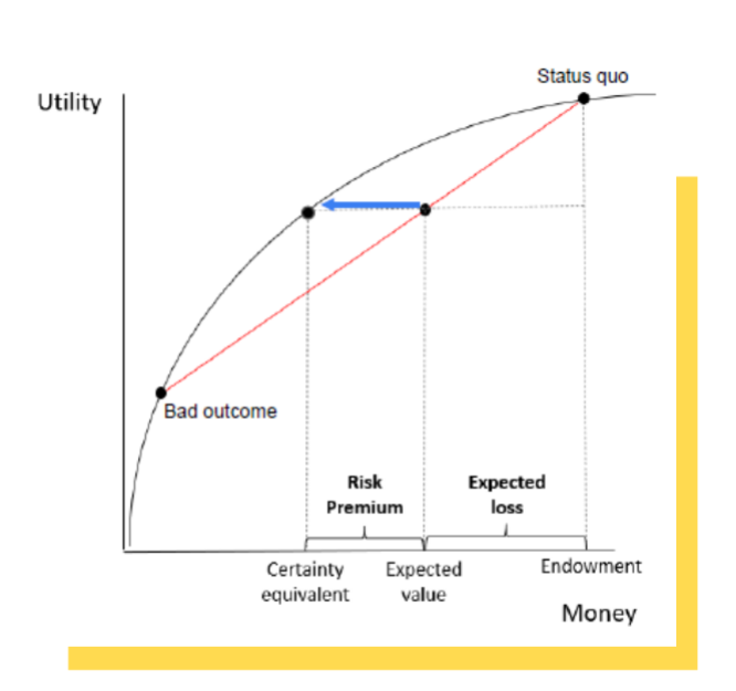
Expected loss

Endowment $ - expected value of money

Utility w/o insurance

Probability of bad outcome x utility of bad outcome + probability of bad outcome x utility of good outcome

Utility w/ insurance

sqrt(Endowment - Insurance Price)

Demand for Insurance

Willingness to pay for insurance = expected loss + risk premium

Supply for insurance

Expected marginal costs to pay claims

Insurance premium

Money that is paid to an insurer so that an individual will be insured against adverse events

Actuarially fair premium

Insurance premium that is set equal to the insurer’s expected payout

Pooling equilibrium

Insurance companies offer a single contract based on average risk

○ PriceA > PriceAVERAGE > PriceH

○ Good deal for ailing types; not so good a deal for healthy types, but maybe still better than no insurance

Separating equilibrium

Insurance companies offer two contracts

○ One expensive contract with full insurance for the ailing

○ One cheaper contract with partial insurance for the healthy

○ Each type self-selects to the intended contract → outcome still not efficient

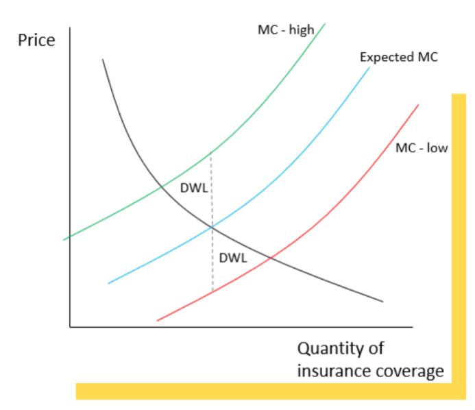
Adverse selection in health insurance

● Insurers can’t tell which consumers will be more/less expensive to insure, so they estimate overall expected cost → single price

● Two areas of DWL are created because the price is too low for high-cost buyers and too high for low-cost buyers.

● It would be more efficient if insurers had enough information to tell which buyers are high-cost vs. low-cost → set separate prices

Death spiral

With adverse selection, market for insurance can “unravel” in a “death spiral”

○ Insurance offered at average fair price

■ bad deal for low risk people and hence only high risk people buy it

■ insurers make losses and are forced to raise the price further

■ only very high risk people buy it

■ insurers make losses again

■ no insurance contract is offered at all, even though everyone wants full actuarially fair insurance

● This inefficiency arises because of asymmetric information

Adverse selection intervention

Policy solution is a mandate - redistribution is needed to solve this

Gov may intervene because healthcare is seen as a right, externalities, paternalism (gov knows better than people do and makes a better choice) and lower administrative costs

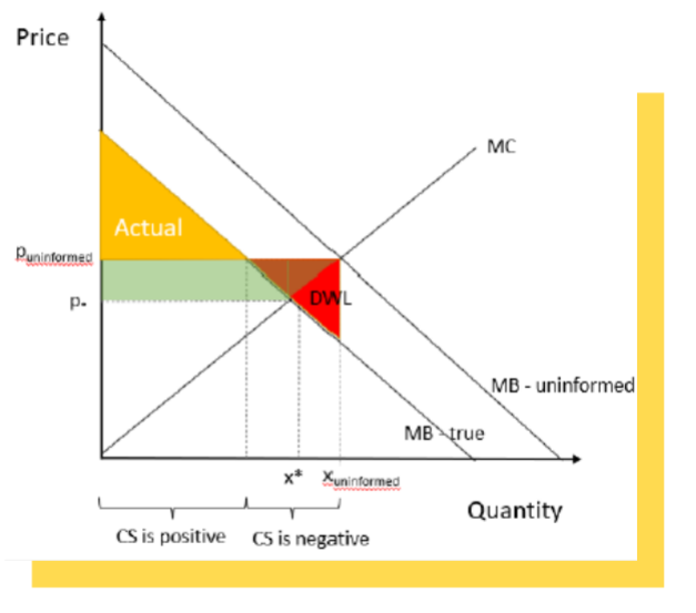
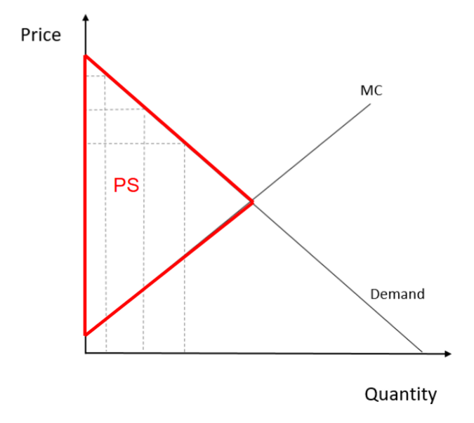
When sellers know more than buyers: Effects on producers’ surplus

● With asymmetric information, sellers

convince buyers that their MB is higher

○ Increasing price and quantity -> adding the

green area to PS

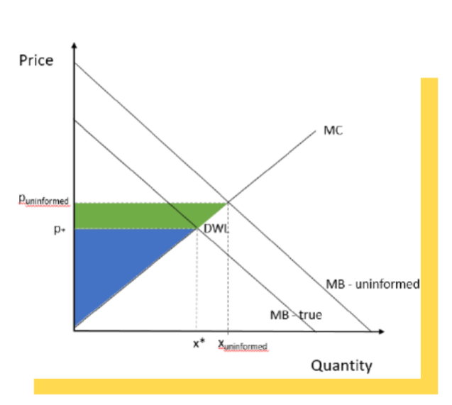
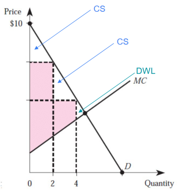
When sellers know more than buyers: Effects on consumers’ surplus

● In a fully informed market -> CS would be the yellow triangle

● If consumers overestimate the benefits, the equilibrium price and quantity will be higher

● When consumers find out the truth -> results in negative CS (red)

● Light green -> surplus (“rents”) that producers extract from consumers because of asymmetric information

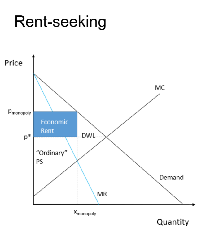
Economic rents

● Income/surplus in excess of what was needed to induce the person to supply labor or

capital

○ Economic rents -> extracting it from other market participants

○ Not Pareto-improving

● Arises from:

○ Naturally arising scarcity rents

○ Policies that interfere with competitive markets

○ Principal-agent problems: adverse selection and moral hazard

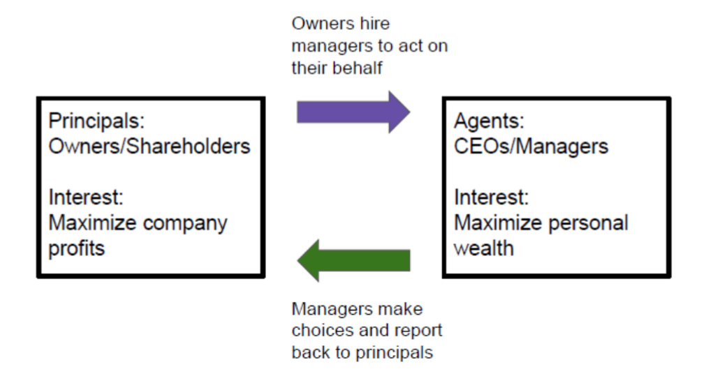
Principal-Agent Problem

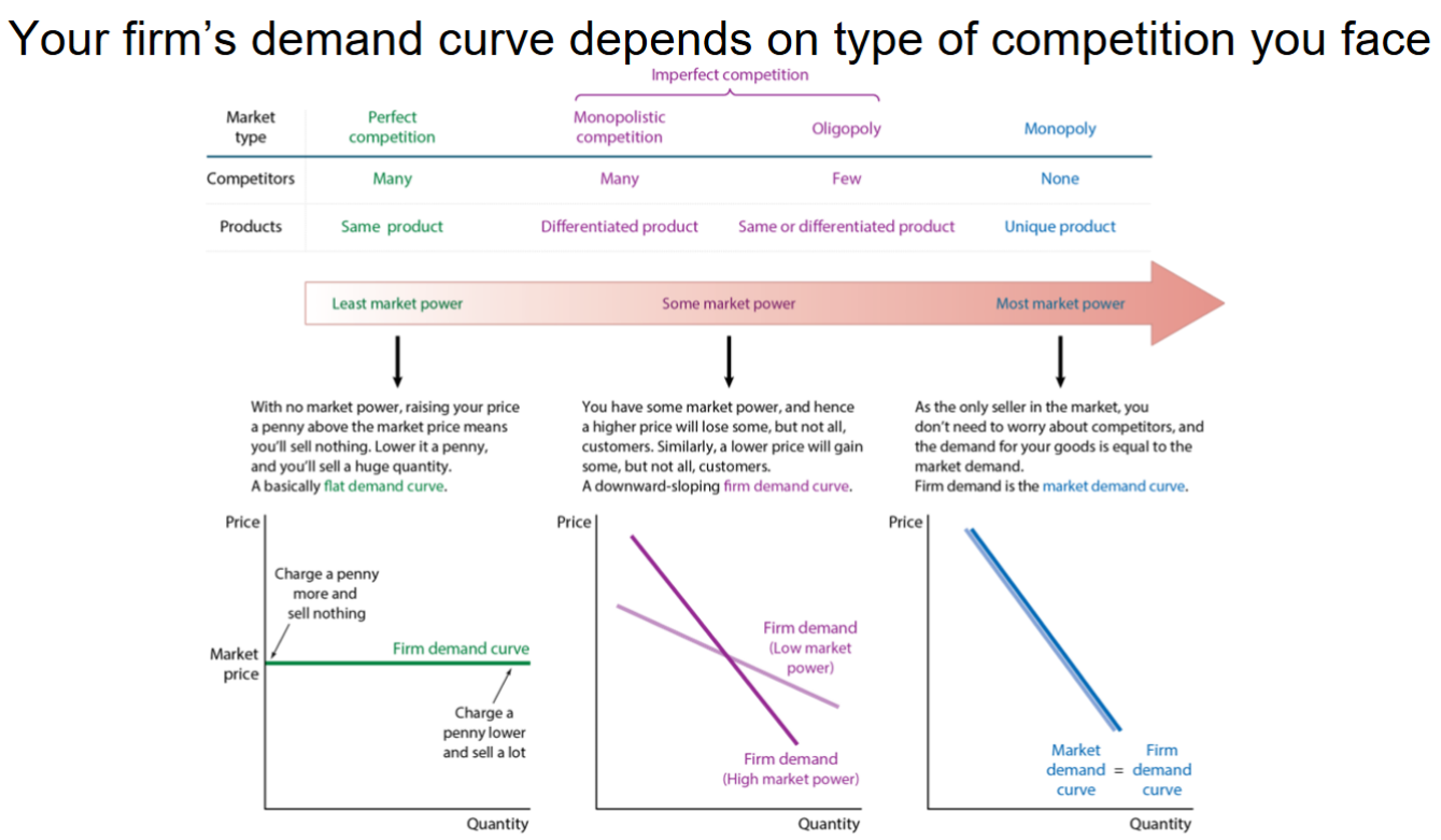
Market power

Extent to which a seller can charge a higher price without losing many sales to competing businesses
Market structure shapes market power

Perfect competition

Many firms, homogeneous products, free entry and exit, no price setting power, price taker influence on price, no advertising (ex: agricultural markets, stock exchange). Pretty rare

Monopolistic competition

Many firms, differentiated products (the more distinct your product is, the less your rivals’ products will be close substitutes), relatively easy entry and exit, limited price setting power, price maker, substantial (ex: fast food chains, clothing brands)

Oligopoly

Few firms, homogeneous or differentiated, restricted entry and exit, limited price setting power, price setter, moderate advertising (ex: automobile industry, airlines, cell phone providers, soft drinks)  

Monopoly

One firm, unique product differentiation, blocked entry and exit, significant price setting power, price maker, variable advertising (ex: local utility companies, Microsoft)

Marginal revenue

● Two competing forces

○ Discount effect: revenue loss from reducing the price on all units sold

■ ΔP*Q, where ΔP is the price cut must offer to sell an additional unit and Q is the total quantity receiving the price cut

○ Output effect: revenue increase from selling one more unit

■ P -> (starting price)

● As quantity increases, the output effect increases profits while the discount effect decreases profits

○ MR= Output effect-discount effect

■ P - (ΔP*Q)

● Profit maximizing quantity: when MR = MC

○ (Perfect competition produce until MB=MC)

● Slope of MR is twice that of a linear Demand Curve

○ Vertical intercept is same as for demand

○ MR = 0 at half the quantity as for demand

Endowment

Starting point - between where money gained = money lost from losing; utility gained from winning < utility lost from losing

Mitigating adverse selection and reduce opportunities for rent-seeking

● Increase marginal tax rates on high incomes

● Require greater transparency regarding details of CEO compensation structure and amounts

● Corporate governance reform – give other stakeholders (e.g., workers) besides stockholders more influence over executive pay decisions

● Higher minimum wages and labor law reform that makes collective bargaining easier

Setting prices to maximize profit

Could sell larger quantity vs making more money on each item

Use the firm demand curve and the marginal revenue curve to

evaluate this trade off

○ Firm demand curve: summarizes the quantity that buyers demand from an

individual firm as it changes it price

■ Firm demand: quantity demanded from your firm

■ Market demand: quantity demanded across all firms

○ Your firm’s market power shapes your firm’s demand curve

True or false - your firm’s demand curve depends on the type of competition you face

True

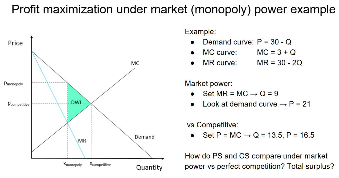
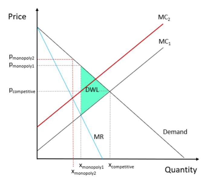
Profit maximization under monopoly

Slope of MR curve is twice that of a

linear Demand curve

○ Vertical intercept is same as for demand

○ MR = 0 at half the quantity as for demand

Compared to competitive equilibrium:

○ Quantity is lower

○ Price is higher

○ Consumers’ surplus is lower

○ Producers’ surplus is higher

○ Deadweight loss

Elasticity and profit margin

Profits go up the more inelastic demand is. Profits go down the more elastic demand is.

Sources of monopoly power

1. Exclusive control over key inputs/raw materials - If a particular firm owns (nearly) all of an input required for production of a particular good or service, then it may emerge as only producer of that good or service (ex: DeBeers diamonds)

2. Natural monopoly - economies of scale

3. Network effects

4. Government-granted monopoly power

a. Intellectual property - Governments give patents to encourage innovation

b. Licenses/Franchises - State and local governments commonly assign exclusive licenses/franchises—rights to conduct business in a specific markets (taxis, charter schools, water, telephone service providers)

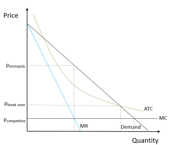
Natural monopoly

Market in which a single business can service the entire market at a lower cost than can multiple businesses (ex: sewerlines, natural gas, electricity)

● Happens when have high fixed costs and/or marginal costs decrease as expand output → average cost of production is declining as output increases

● Economies of scale mean that over the relevant quantity range:

○ Average total cost is declining

○ MC < ATC

○ Usually due to high fixed costs, but can also be caused by declining variable costs or economies of scope

● P = MC maximizes welfare

● But when P < ATC, revenue doesn’t

cover cost, so firms lose money

● Social optimum is not possible

● Subsidize production

● “Rate of return” regulation

● Attempts to set price at break even + “fair” rate of return on capital

● Allow price discrimination

○ “Peak load pricing” is intertemporal price discrimination

● Public enterprise

If gov provides services - P = MC, uses tax revenues to pay for losses

Network effects

Arise in situations where products become more useful/valuable the larger the number of users of the product (Blu-Ray, cars from major companies as mechanics will have more parts and better experience, social media)

Consequences of Market Power - Rent-seeking

Monopolists have an incentive to engage in anti-competitive behaviors or spend on lobbyists/ accountants/ lawyers to protect their access to economic rents

Consequences of Market Power - X-inefficiency

X-inefficiency - monopolist’s production costs may drift upward due to lack of competitive pressure →

○ Price increases

○ Quantity decreases

○ DWL increases

(Higher production cost than necessary for output)

Creative destruction

The idea that firms have an incentive to innovate in order to become monopolists, and then are eventually replaced by an even more innovative monopolist

Incentive to innovate / relationship between competition and innovation

○ Too little competition and monopolist has no incentive to innovate to keep market position

○ Too much competition and the potential returns to innovation are small (other firms will quickly leapfrog)

First Degree / Perfect Price Discrimination

Assumptions

1. The monopolist can charge individual prices

2. The monopolist observes the entire demand curve

3. No arbitrage or resale

● Each consumer is charged their willingness to pay (i.e., personalized pricing)

● All consumer surplus goes to producers
Examples include haggling and collecting data to understand true WTP

Second Degree Price Discrimination

● Sellers do not have enough information to perfectly price discriminate

● Set different prices for consumers based on how much they are consuming

● E.g., quantity discounts

○ BOGO

○ “Buy 1 get 1 50% off”

○ Discounts for medium, large drinks
● Producers are able to extract rents from consumers

● Consumers still get some surplus

● There is still some deadweight loss

● Smaller than single price monopoly

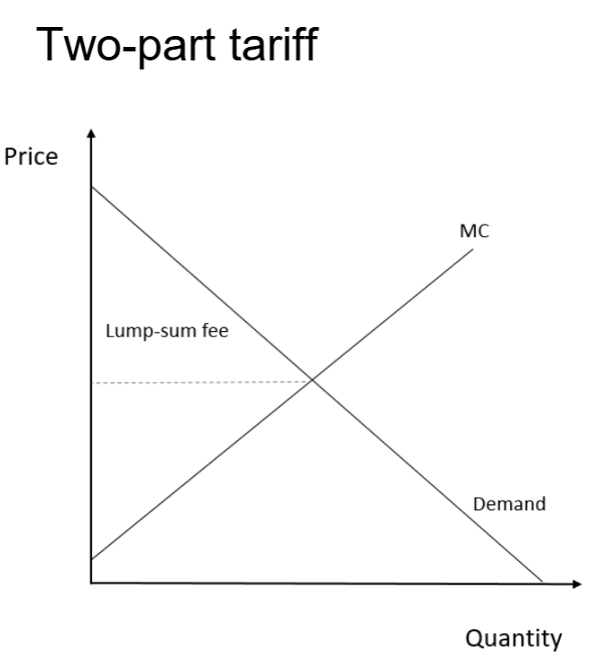
Two part tariff

● Combine a fixed upfront fee with a per-unit price

● Set the per-unit price competitively, where MB = MC

● Create a lump-sum fee equal to the entire

consumers’ surplus

● All surplus goes to the producers

● Examples

○ Admission fee + per-ride fee

○ Gym membership + per-class fee

○ Monthly internet/phone subscription + per GB fee

Third Degree Price Discrimination

● Producers “segment” consumers into different groups based on observable/verifiable characteristics

● Producers operate as single-price monopolists in each segment

● E.g., domestic and international versions of textbooks; movie tickets (students/senior citizens vs others)

● There is still deadweight loss

● But, there is less deadweight loss than with a single price monopolist

Is monopoly/market power inherently bad?

● Not all monopolists practice anti-competitive behaviors

● Restraint of trade

● Predatory pricing

● Anti-competitive mergers or acquisitions

● Monopolists can use their profit in ways that benefit consumers

○ Innovation and basic science research

○ Product development

● Sometimes a monopolist can supply a good at a lower cost than two or more suppliers → natural monopoly

● Monopolists generally make money by restricting quantity, so they could offset the overproduction of goods with negative externalities

Justification for Public Policy - Efficiency

● Economic theory defines efficiency maximization as a normative goal

○ Is total efficiency/surplus maximized? Is the “pie” as big as possible?

○ Is deadweight loss minimized or eliminated?

○ Are all mutually beneficial gains from trade exhausted?

● Provides justification for government intervention in cases of market failure

Justification for Public Policy - Distributional Equity

● Defining equity goals is not typically part of normative economic theory

● All else equal, any redistribution should have the least possible effect on efficiency (or increase it, if possible)

● Economic tools like welfare analysis and econometrics can be used to measure distributional outcomes and identify causal mechanisms

Distributional equity is about outcomes (resource allocations), not procedures (rules/decision processes to determine outcomes)

Social Welfare Function - Utilitarian

W = U 1 + U 2 + U 3 + ... Provides an efficiency-based justification for redistribution if we assume there is diminishing marginal utility of income/wealth

Social Welfare Function - Rawlsian

W = min(U1 , U2 , U3 , ...)

○ Social welfare determined entirely by the well-being of the worst-off person in society

○ Provides a justification for any redistribution that increases the utility of the least well-off person in society

Horizontal equity

Individuals with similar incomes should be treated similarly by the tax system

Vertical equity

Groups with more resources should pay higher taxes than groups with few resources

Cash transfers

○ Temporary Assistance for Needy Families (TANF): provides support to low-income families with children; 5-year lifetime limit and requires transfer recipients to work after 24 months

○ Supplemental Security Income (SSI): transfers to individuals who are aged, blind, or have a disability

○ Earned Income Tax Credit (EITC): refundable tax credit for low- to moderate-income working individuals and couples

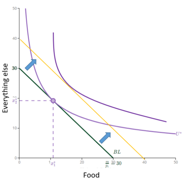
Explanation of graph:

● Use composite good (“everything else”) for Good 2

● Cash transfer results in parallel shift in budget constraint

● Pure income effect

● If food is a normal good, you will consume more of it

● Will consumers spend the entire transfer on more food?

● Depends on preferences

In-kind transfers

○ Supplemental Nutrition Assistance Program (SNAP), Special Supplemental Nutrition Program for Women, Infants, and Children (WIC)

○ Medicaid

○ Public housing

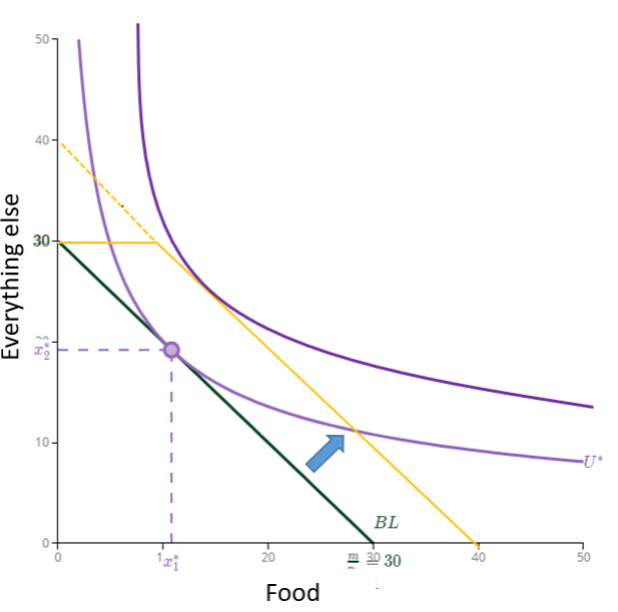
Explanation of graph:

● Assume benefit = $10 of food, results in “kinked” budget

● Pure income effect

● For some, the optimal choice is the same as if they got $10 in cash instead

● Others would be better off if they got cash instead

● For this consumer, food is an inferior good

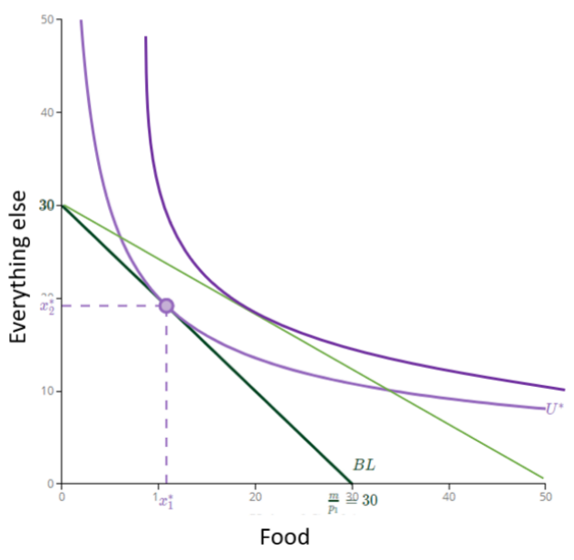
Subsidies

● Subsidy reduces the price of food and rotates the budget constraint

○ Substitution effect: Food is cheaper so you buy more

○ Income effect: Your budget set is larger, so you buy more normal goods

● Will consumers buy more/less of everything else?

○ Depends on preferences

Cost of redistribution

1. Costs of administration

2. Behavioral response of those being taxed

○ E.g., higher income individuals taxed to pay for income transfers

○ Taxation lowers returns to work, may cause higher income people to work less

3. Moral hazard behavioral response

○ As government insures individuals against being poor, raises incentive for individuals to be categorized as poor in order to qualify for these transfers

○ Raises cost of providing those transfers

Demand Curve

● “At each price, how many will the consumer buy?”

● Traces out all of the consumer’s utility-maximizing quantity choices at every possible price.

DUAL INTERPRETATION: “At each quantity, what’s your marginal benefit?”

Law of Demand

○ As price ↑, quantity ↓

○ Demand curves slope downward

DUAL INTERPRETATION:

As quantity increases, willingness to pay (MB) decreases because of diminishing marginal utility

Marginal Benefit (MB)

Willingness to Pay, marginal utility expressed in $

Demand Curve Shifters

● Changes in consumer preferences

○ Policy examples: consumer disclosure policies (e.g., nutrition facts on food)

● Changes in consumer income - normal or inferior good

○ Policy examples: Income tax policy, universal basic income policies

● Changes in prices of complements or substitutes

○ Policy example: Subsidizing higher education expands the demand for student housing

● Changes in expectations about the future

○ Policy examples: Fed signaling monetary policy, major investments in infrastructure

● Changes in the number of consumers

○ Policy example: ACA mandates purchase of health insurance

Decrease - demand shifts inward; increase - demand shifts outward

True or false: Changes in price shift the demand curve

False - change in price changes the quantity demanded

Arc elasticity formula

Elasticity = percentage change in quantity / percentage change in price

Elasticity = (X2 - X1)/(X1+X2/2) / (P2 - P1)/(P1+P2/2)

Measures how receptive buyers / sellers are to price changes

How would you interpret a price elasticity of demand that’s -1.6?

A 1% increase (decrease) in price leads to a 1.6% decrease (increase) in quantity demanded. No units.

Larger magnitude = consumers are more responsive to price (or opposite - more responsive sellers are to price changes)

Elastic vs inelastic vs unit elastic demand

● Absolute value of the price elasticity is greater than 1 → Demand is “elastic”

○ The percent change in quantity is larger than the percent change in price

○ Quantity is “very” responsive to changes in price

○ Demand curve is relatively flat

● Absolute value of the price elasticity is less than 1 → Demand is “inelastic”

○ The percent change in quantity is smaller than the percent change in price

○ Quantity is “not very” responsive to changes in price

○ Demand curve is relatively steep

● Absolute value of the price elasticity is equal to 1 → Demand is “unit elastic” (total revenue remains unchanged)

What factors affect the price elasticity of demand?

Inelastic (lower elasticity) Elastic (higher elasticity)

Necessities Luxuries

Categories Specific brands

Short time horizon Longer time horizon

Low willingness to search for substitutes High willingness to search for substitutes

Supply curve

● Traces out a firm’s profit-maximizing quantity at each possible price

● As the price gets higher, firms have stronger incentives to put more resources into production and try to sell more

DUAL INTERPRETATION
“At each quantity, what is the marginal cost?”

Law of Supply

The higher the price, the greater the quantity supplied

DUAL INTERPRETATION
As quantity increases, marginal costs increase because of diminishing marginal productivity of inputs

Supply Curve Shifters

● Changes in costs

○ Technology, production processes, input prices - e.g., wages for labor, price of rent, etc.

○ Policy examples: R&D subsidies, tax breaks, minimum wage, environmental regulations

● Changes in producer expectations about prices

○ If prices are expected to rise/fall in the future, firms may preemptively expand/reduce production

○ Policy examples: Federal Reserve signals about monetary policy, major investments in infrastructure

● Changes in number of producers

○ More businesses, higher total production; Fewer businesses, lower total production

○ Policy examples: business licensing, entrepreneurship support

Cheaper production - supply shifts out (increases)

More expensive production - supply shifts in (decreases)

What factors affect price elasticities of supply?

Depends on how flexible businesses can be

● Larger in the following circumstances:

○ For firms that store inventories

○ When inputs are easily available

○ For firms with extra capacity

○ When firms can easily enter and exit the market

Market Equilibrium

Price at which the quantity buyers want to buy = price at which the quantity sellers want to sell

MC = MB - trade stops here

Market will always tend toward equilibrium

Shortage

Price is too low - quantity demanded > quantity supplied

Buyers bid up the price / secondary market appears

Sellers have an incentive to expand output as prices increase

Surplus

Price is too high - quantity supplied > quantity demanded

Sellers need to get rid of excess by putting it on sale

Sellers have an incentive to reduce output as price falls

Total Expenditure

TE = Price * Quantity

Total Benefit (area under demand curve)

TB = Area under demand curve

Consumer surplus (in relation to TB & TE)

CS = TB - TE

Total revenue

TR = Price * Quantity

Total cost

TC = Area under supply curve

Producer surplus (in relation to TR & TC)

PS = TR - TC

Total surplus

CS + PS

Deadweight Loss

Destruction of value as a result of a market being out of equilibrium (i.e., “inefficiency”)

Assumptions of perfectly competitive markets

1. Agents are “rational”

○ Consumers maximize utility subject to budget constraints

○ Firms maximize profits subject to production costs

2. Perfect information and instantaneous decisions

3. Large numbers of buyers and sellers

4. Product homogeneity (selling identical goods)

5. “Frictionless” markets – free entry/exit and no transaction costs

6. No externalities

First Fundamental Theorem of Welfare Economics

● If assumptions of perfect competition are met, the competitive market equilibrium is “Pareto efficient”

○ Cannot increase anyone’s surplus without reducing someone else’s

○ All mutually beneficial trades have been made; no DWL

● Government intervention may be particularly desirable if

perfect competition assumptions fail, i.e., when there are

market failures

→ Govt intervention can potentially improve everyone’s welfare

What Pareto efficient does not mean

● Distribution of initial resources is “fair”

● Resulting distribution of purchased goods/services is “fair”

● Economics processes are “fair”

● Preferences are “good” or socially desirable

● There’s only one possible Pareto efficient outcome (there can be many)

Even with no market failures, competitive market outcome may generate substantial inequality

Second Fundamental Theorem of Welfare Economics

● Any Pareto-optimal outcome can be reached with competitive markets, provided the right redistribution of initial wealth/resources [lump-sum taxes based on individual characteristics and not behavior]

● In reality, 2nd welfare theorem does not work because redistribution of initial endowments is not feasible

○ Initial endowments difficult for the government to observe

○ Govt needs to use distortionary taxes and transfers based on

economic outcomes (such as income or working situation)

→ Conflict between efficiency and equity: Equity-Efficiency trade-off

Economic Rules of Rational Behavior

1. Every choice can be measured in terms of utility

2. Resources are scarce and scarcity requires tradeoffs

3. People try to maximize their utility subject to resource

constraints (cost/benefit thinking)

4. People make choices “on the margin”

→ Economic “rationality” is about the decision

process, not the inputs or outcomes

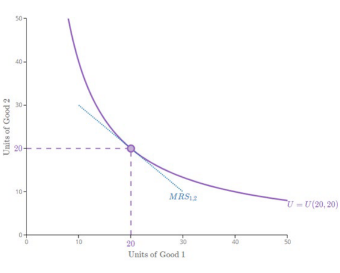
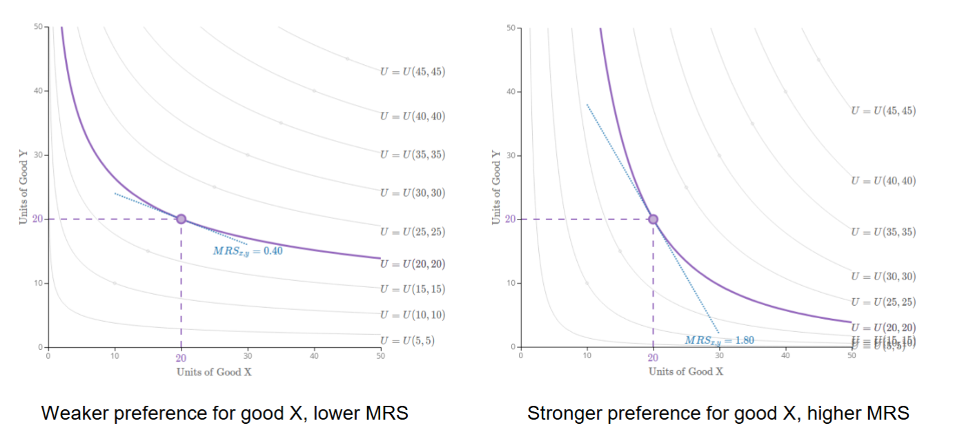
Marginal Rate of Substitution

MRS = MU1 / MU2

● MRS = amount of Good 2 you would give up to get one more unit of Good 1, while maintaining same utility

● Negative slope

● MRS has a unique value at every point along the I.C.

● Diminishing MRS → convex I.C.s

Optimal choice is where MRS = p1/p2. Internal rate of tradeoff MRS = market rate of tradeoff (price ratio)

Low vs High MRS

Left graph - flatter curve, doesn’t care about good X as much, would only give up a small amount of Y for X

Right graph - steeper curve, would give up a lot of Y for X, value X, would give up 1.8 units for X

Normal vs inferior good

What’s a normal vs inferior good depends on preferences. If income goes up and quantity goes up it’s a normal good. If income goes up and quantity goes down it’s an inferior good.

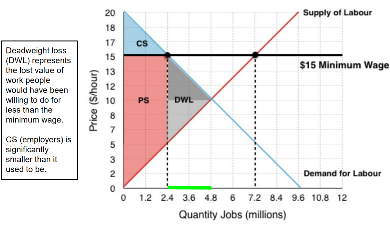
Minimum wage as a price floor: Neoclassical theory

Price floor policy: Requires a price above equilibrium in the market for unskilled labor

Quantity reduction: in green, a result of moving along the labor demand curve

Unemployment: Excess supply/surplus of workers created by price ceiling

In general, PS (workers) may go up or down. Workers lose

some surplus to DWL but gain surplus that used to be consumers’ (i.e., employers’) surplus.

Differences in differences model

A quasi-experimental economic method for estimating the causal impact of an intervention by comparing the change in outcomes over time between a treated group and a control group. It relies on the "parallel trends" assumption, which states that the outcome for both groups would have followed a similar trend in the absence of the treatment. The method is calculated by subtracting the change in the control group's outcome from the change in the treated group's outcome over two periods (pre- and post-intervention).

True or false - economic cost = opportunity cost

True

Standing

Whose cost counts or gets counted? Whose benefits get counted?

Valuation Method - Revealed Preference (market-based)

● Examine actual market data for related goods/services and extrapolate to the good/service in question (e.g., “green” products)

● Hedonic price analysis looks at values for homes with different features or amenities (e.g., proximity to transit)

● Hedonic wage analysis looks at wages for different jobs (e.g., jobs that are dangerous)

Valuation Method - Stated Preference / Contingent Valuation

● Uses surveys to ask people their willingness to pay/accept

● Questions can be yes/no: “Would you be willing to pay $X for _____?”

● Questions can be open-ended: “How much would you be willing to pay for _____?”