STAT115 equations

+ like what they mean yk

Ratio

Fraction of one quantity over another.

E.g. class 10 boys, 20 girls - ratio boys to girls = 10/2 = ½ = 0.5 Girls to boys = 20/10 = 2

Proportion

Fraction of one quantity compared to the whole

E.g. class 10 boys, 20 girls. Proportion of boys = 10/(10+20) = 1/3. Proportion of girls = 20/(10+20) = 2/3

To convert proportions to percentages

x 100, add % sign

To convert percentages to proportions

Divide by 100, remove % sign

Mean equation (2 possibilities)

• ȳ = mean

• y1, y2, yn, etc = data points for patient 1, 2, n (however many numbers)

• n = total sample size

OR

• Σ = Sigma, summation operator, sum sequence of terms (up to value n, usually total sample size)

• i = 1 means start at the first value

• e.g. i = 3 in this equation would mean y1+y2+y3

• yi = a value (y1, y2, etc)

• n = sample size aka total amount of values

Sample variance equation

average squared distance between observations and the mean.

If an observation (yi) is far from mean (ybar), (yi-ybar)² will be large, s² will be large

• Σ = summation operator, sum things (up to n value, data set size usually).

• i = starting value (usually 1st value, 1)

• yi = a value (y1, y2, etc)

• ybar = mean

• n = sample size aka total amount of values

Standard deviation equation

Square root of variance (previous flashcard)

• Approximately 70% of the data will be within one standard deviation of the mean

• Approximately 95% of the data will be within two standard deviations of the mean 

• don’t hold if data skewed or multimodal

Probability

Between 0 and 1, probabilities sum to 1. Probability of an outcome is the proportion of times outcome occurs if were to observe the random process an infinite number of times.

Probability for mutually exclusive outcomes (cannot both happen)

Pr(A or B) = Pr(A) + Pr(B)

• Pr(A or B) is inclusive, means that either A, B, or both A and B occur

• For mutually exclusive events, Pr(A and B) = 0 (general addition rule has - Pr(A and B) at the end)

Probability for events that are not mutually exclusive (removes overlap)

Pr(A or B) = Pr(A) + Pr(B) - Pr(A and B)

• Pr(A or B) is inclusive, means that either A, B, or both A and B occur

E.g. Event A = rolling 1, 2, 3, 4. Event B = rolling 1, 3, 5. (six sided dice)

Pr(A or B) = 4/6 + 3/6 - 2/6 = 5/6

e.g. Pr(seen by at least 1 detector) = 1 - Pr(not seen by any detector)

Complement equation

Outcomes that are not in an event.

Pr(A) + Pr(A∁) = 1

Pr(A) = 1 - Pr(A∁)

Probability of independent events occurring together

Independent events = outcome of one event provides no info about outcome of the other (doesn’t influence each other).

Pr(A and B) = Pr(A) x Pr(B)

Conditional probability

Pr(B|A) = Pr(A and B) / Pr(A)

• Relationship between 2 events

• Probability of event B given event A has occurred = Pr (B|A)

Conditional probability for independent events

Pr(B|A) = Pr(B)

• Event A occurring does not change the probability of event B occurring

• Pr(B|A) = (Pr(A) x Pr(B)) / Pr(A)

• So Pr(A) cancels itself out

• Probability of a single event = marginal probability (e.g. Pr(A))

Pr(A and B) for independent events - probability of A and B occurring (general multiplication rule)

Pr(A and B) = Pr(A)*Pr(B)

Pr(A and B) for dependent events - probability of A and B occurring (general multiplication rule)

Pr(A and B) = Pr(B|A)*Pr(A)

• Can also switch A and B, so Pr(A and B) = Pr(A|B)*Pr(B)

Contingency tables

Compare 2 categorical values. Proportions are found by dividing entries by total.

• Pr(M and S) = 0.162 

• Pr(M and S^∁ ) = 0.635

• Pr(M^∁ and S) = 0.151 

• Pr(M^∁ and S^∁ ) = 0.052

• M^∁ = not being male (aka being female), S^∁ = didn’t survive

Conditional probabilities for contingency tables (titanic example) - looking at rows

• Probability of surviving given you’re male: Pr(S|M) = Pr(S and M) / Pr(M) = 0.162/0.797 = 0.20

• Probability of surviving given you’re not male (female): Pr(S|M^∁) = 0.151/0.203 = 0.74

Example for multiplication rule aka Pr(A and B)

•  “96.1% of the residents were not inoculated, and 85.9% of the residents who were not inoculated ended up surviving.”

• What is the probability that a resident was not inoculated (A) and lived (B)?

Pr(A and B) = Pr(0.961)*Pr(0.859 | 0.961) = 0.961 × 0.859 = 0.825

• Pr(A) (0.961) cancelled itself out in Pr(B|A)

Order doesn’t matter for joint probability

Pr(A and B) = Pr(B and A)

Order does matter for the conditional probability

Pr(A | B) and Pr(B | A) are two different quantities

A given B occurred, or B given A occurred

Finding marginal probability (probability of a single event): law of total probability

• To find e.g. Pr(B), sum possible outcomes that could co-occur with the event B

• If there are 2 outcomes: A1, and A2 (aka A1^∁, complement of A1)

Pr(B) = Pr(A1 and B) + Pr(A1^∁ and B)

• Could also write A1^∁ as A2

Tree diagrams (alternative way to visualise data other than contingency tables, for conditional probability questions)

Example:

• Pr(I and L) = 0.039×0.975 = 0.038

Bayes’ theorem - finding Pr(A|B) from Pr(B|A)

Rearranging to find A given B from B given A.

Example of Bayes’ theorem - finding Pr(A|B) from Pr(B|A)

• 90% of patients with sleep apnea snore: Pr(S | A) = 0.9 

• 50% of patients without sleep apnea snore: Pr(S | A∁ ) = 0.5 

• 5% of the population have sleep apnea: Pr(A) = 0.05

  

• Pr(S | A) = 0.9 (snore given you have sleep apnea)

  • Tempting to think that Pr(A | S) will also be high (have sleep apnea given you snore)

  • Pr(A | S) ≈ 0.09 seems surprisingly low 

• In the general population, we have

  • Pr(A) = 0.05

• After learning that patient snores, the probability increases to

  • Pr(A | S) ≈ 0.09

Random variable

A random variable assigns a numerical value to each outcome in sample space, aka A random variable is a (random) process with a numerical outcome

• Common to represent a random variable with capital letter

  • e.g. X or Y or Z

• The possible values are given with lowercase letters 

  • e.g. x, y, z

e.g. Y = number of farms with evidence of leptospira.

If you visit 3 farms, four possible values: y1 = 0, y2 = 1, y3 = 2, y4 = 3 (no farms have it up to all 3 farms having it)

Visit 30 farms, 31 possible values: y1 = 0, y2 = 1, …. y31 = 30.

• We may use i (or j) as an index of possible values

  • e.g. i = 2 is the second possible value; yi = y2 = 1

• Use k to represent number of possible values

  • k = 4 if we visit three farms

  • k = 31 if we visit 30 farms

Probability distribution (probability of a random variable having a certain value)

Pr(Y = yi), probability of random variable (Y) taking the value yi

e.g.

for i = 3 (3rd possible value, which is 2 farms having the disease in this example, if you visited 3 farms): Pr(Y = 2) = 0.4, probability that Y takes the value 2

__

Note: yi doesn’t always have to be 1 value behind i. e.g. if have an online shop:

• With probability 0.4 buy nothing: we receive $0 

• With probability 0.3 buy item A: we receive $20 

• With probability 0.2 buy item B: we receive $35 

• With probability 0.1 buy item A and B: we receive $50

  

• How likely is it that we will receive $20 or below from an online visitor? (mutually exclusive events)

• Pr(Y ≤ 20) = Pr(Y = 0 or Y = 20) = Pr(Y = 0) + Pr(Y = 20) = 0.4 + 0.3 = 0.7

Finding expected value (aka mean) of a random variable

• ∑ means sum all the values up

• Y = random variable, yi = potential value

• i = 1 means start at first value

• k = total number of values/outcomes (I think)

  E[Y] = y1*Pr(Y = y1) + y2*Pr(Y = y2) + y3*Pr(Y = y3) + y4*Pr(Y = y4)

Example:

•  How many farms would we expect to have evidence of leptospira?

Expect 1.55 farms to have evidence of infection (isn’t logical irl but like it’s maths)

• How much money do we expect to receive from an online visitor?

  

Expect to receive $18 on average from a shopper

Also:

• If we saw 100 online visitors

  • We would expect 40 of them to spend nothing: receive $0 

  • We would expect 30 of them to spend $20: receive $600 

  • We would expect 20 of them to spend $35: receive $700 

  • We would expect 10 of them to spend $50: receive $500

Variance (for random variables)

Used for larger problems (rather than probability distribution)

• ∑ means sum all the values up

• i = 1 means start at first value (the 1st possible value)

• k = total number of values

• yi = a potential value of the random variable

• E[Y] = expected value aka mean

Example:

Standard deviation (for combinations of random variables)

Square root of variance is (approximately) the average deviation from the mean 

Example:

Continuous random variables (previously looking at discrete random variables)

Infinite number of possible values, each value has a probability density. Curve = probability density function, probability is given by the area under the curve. Total area under the curve = 1.

e.g.

The probability of systolic blood pressure 125 and 130 mmHg is given by:

• Suppose we know the probability that systolic blood pressure is less than 130 mm (blue)

  • Pr(systolic pressure < 130) = 0.78

•  What is Pr(systolic pressure > 130)? (gold)

  • It is a complement!

  • 130 up to positive infinity

  • So must be 0.22 (complement to 0.78, total area under curve = 1)

(Linear) Combinations of random variables

aX + bY

(variable X and variable Y)

• a and b represent amounts of those variables, can be positive or negative

• e.g. for shares example, If we owned shares: 5 SPK and 10 POT, linear combination represents the value of our portfolio in one month’s time, 5X + 10Y

  • a = number of SPK shares, b = number of POT shares

• For ice cream example, X is amount of ice cream in container, Y is amount in a scoop of icecream (being taken out of the container), so a = +1, b = -1, results in X - Y.

Expected value of combinations of random variables

• If we owned shares: 5 SPK and 10 POT

  • Linear combination represents the value of our portfolio in one month’s time 

  • 5X + 10Y

• How do we find the expected value of the linear combination?

  • E[aX + bY] = aE[X] + bE[Y]

• If E[X] = 3 and E[Y] = 6.3 (mean values of each) then, the expected portfolio value is

  • E[5X + 10Y] = 5E[X] + 10E[Y]

    • 5 × 3 + 10 × 6.3

    • = 78

For ice cream example, where a = +1 and b = -1, equation is E[X - Y] = E[X] - E[Y]

Variance of combinations of random variables (if they are independent)

variables = X and Y, independent

previous flashcards have info on a and b

Abstract example of expected value (mean) and variance of a combination of independent random variables

• Let Y1 and Y2 be independent observations from a distribution

  • Mean µ 

  • Standard deviation σ

• What is the expected value and variance of (Y1 + Y2) / 2 (sample mean)?

Expected value of sample mean:

(a and b in this are both 1/2)

Variance of sample mean:

Can be extended to when we have more than 2 independent observations:

How to write that a variable follows a normal distribution/normal model

C~Normal(µ, σ²)

• in this example, the variable is “C”

• C distributed as a normal distribution, defined by a mean (µ) and variance (σ²) (or sometimes standard deviation, σ)

Normal model/normal distribution

Bell-shaped curve aka Gaussian model - symmetric, continuous

Described by mean (µ) and standard deviation (σ) (or sometimes variance, σ²)

• N(µ, σ) or N(µ,σ²)

By default, mean is zero and standard deviation is 1

Model fitting

µˆ = ¯y           population mean = sample mean

σˆ = s            population st dev = sample st dev

Population mean or standard deviation being estimated by the sample mean or standard deviation (they aren’t the exact same, can change depending on the sample, population values can’t be exactly known as can’t sample the entire population).

making continuous data fit a normal distribution if it’s skewed - transformations

Data (especially positive) often have skewed distribution - not symmetric.

Using log-transform (logarithm) can make data more normally distributed, e.g. use variable log(y) rather than y

Probability density function

Likelihood of a continuous random variable being a particular value or being within a range of values.

Total area under the curve = 1.

Pr(Y greater than or equal to y) = area

• for a specific section of the curve

• Y (capital) is the random variable, y is a potential value it could take.

z-score (normal distributions)

How many standard deviations above the mean a value is (z = 1 means value is 1 standard deviation about the mean)

y = potential value, µ = mean, σ = standard deviation

example for IQ test (IQ of 115, mean 100, standard deviation 15):

find y (potential value of a continuous random variable) from a z-score (normal distribution)

y = µ + zσ

• µ = mean, σ = standard deviation

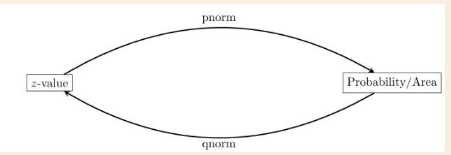
R functions for normal distributions

• dnorm: density function 

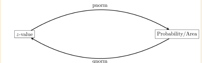
• pnorm: probability function 

• qnorm: quantile function 

• rnorm: generate random values

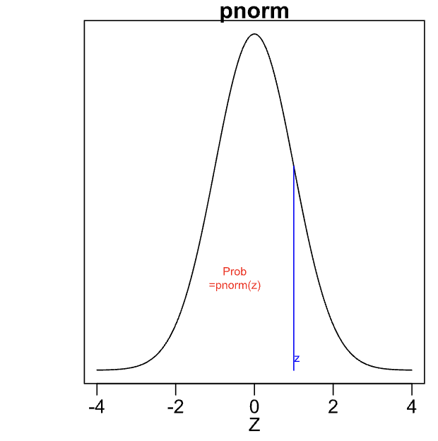
probability that a random variable value is less than a given value, more than, or between 2 values (normal distribution) - probability function

aka converting a z-score to a probability/area

pnorm(q)

• probability function of value “q”

Pr(Z < q)

• Z = z-score

pnorm(q) = area = Pr(Z < q)

mu = mean, sigma = standard deviation

find z-score, then do pnorm stuff:

e.g. what is the probability that IQ is less than 85 (mean of 100, sd of 15)

Probability that IQ is more than 120?

Probability that IQ is between 110 and 130?

percentage of values within standard deviations of the mean (normal distribution)

Z = z-score

•  Pr(−1 < Z < 1) = 0.6827

  • Approximately 68% of values should be within 1 sd of the mean

• Pr(−2 < Z < 2) = 0.9545

  • Approximately 95% of values should be within 2 sd of the mean

• Pr(−3 < Z < 3) = 0.9973

  •  More than 99% of values should be within 3 sd of the mean

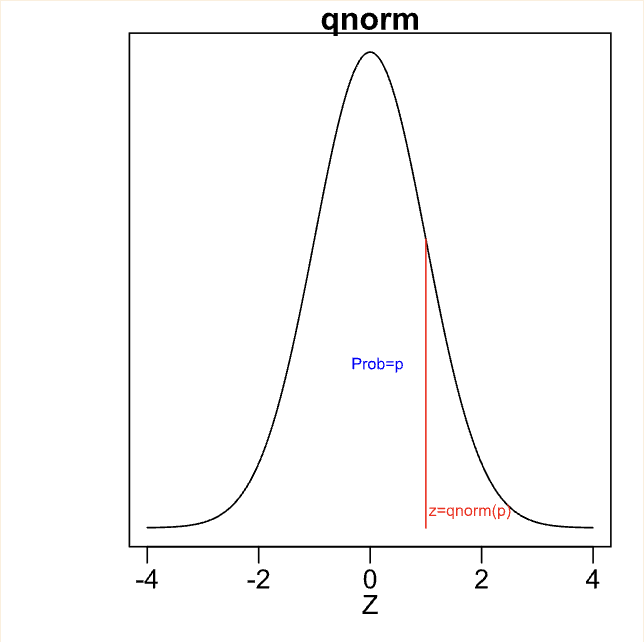
quantile function, qnorm (finding z-score for known value/percentage aka probability/area, normal distribution)

• The value q is given by qnorm(p)

  • The value of p is the black area (known)

qnorm(value) = z-score

example (from prac assignment 3):

Find reaction times which the central 97% of people fall between. Calculate the upper and lower limit of this range. That is, find the reaction time which 1.5% of people are faster than, and the reaction time which 1.5% of people are slower than.

• Find the z-value for the time which 1.5% of people’s reaction times are faster (i.e. lower) than. This z-value can be found using qnorm(0.015), which equals -2.1701 (when rounded to 4 DP) (this is the actual qnorm part, finds the z-score, next part finds the actual value from the z-score)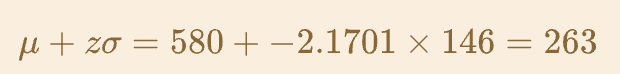

  • 

  • 1.5% of inds are faster/lower than 263ms

• Find the -value for the time which 1.5% of people’s reaction times are slower (i.e. greater) than. This will be the z-value for the time which (100-1.5)% = 98.5% of people’s reaction times are faster (i.e. less) than.

  • This -value can be found using qnorm(0.985), which equals 2.1701 (when rounded to 4 DP).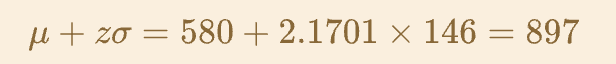

  • 

  • 1.5% of inds are slower/greater than 897ms

estimating sample mean (ybar) from a sample if we knew the population mean and sd

randomly generated sample mean from sample size of n - different to true population mean of 2.45

sampling distribution - how statistics (e.g. sample mean aka ybar aka y¯) vary from one sample to another

e.g. from example of normal distribution (tested a bunch of samples using R)

(above to create values for below graph)

- On average it is 2.45: the value of µ

• Sample means less than 2.35 or larger than 2.55 are unlikely

• Could use R to count how many samples (of 10 000) had mean less than 2.36

  

note: for estimating how extreme a sample mean is (chance of observing a sample mean as extreme as a value), have to do both top and bottom of distribution

expected value of a mean of a normal distribution - expected value mean of the sampling distribution

E[(y1 +y2)/2] = ½[E(y1) + E(y2)] = ½[µ + µ] = ½ x 2µ = µ

• Expected value of mean of 2 values in the sample is the mean of the sampling distribution

example: What is the chance of observing a sample mean as extreme as y¯ = 2.36?, If the µ = 2.45 and σ = 0.75?

• 1. Find mean and sd of sampling distribution

• 2. Convert to z-value

• 3. Find the probability

Z = (2.36 - 2.45) / 0.75/√314 = -2.021

note: if n is small (n = 1, sample size), sample mean is the same as an observation, same sd. If n is large (n = 1 000 000), sd of sample mean is 1/1000th the sd of observations

Variance of a sampling distribution (normal distribution)

var(ybar) = var(y1 + y2 + y3 + … yn / n) = 1/n^2 [Var(y1) +var(y2) + … var(yn)] = 1/σ^2(σ^2 + σ^2 + … +σ ^2)

• Variance of y1 = σ^2

• sample standard deviation is σ / √ n

Standard error of sample mean (sampling distribution, normal distribution)

σ/√n

• σ = (population) standard deviation

• n = sample size

probability of finding a more extreme sample mean than a given value (sampling distributions, normal distribution)

find z-score (with standard deviation being the given standard error), then pnorm of z-score (calculation depends on if asking for greater or less than value), then times that value by 2 (finding both upper and lower tail)

pnorm(answer of above)

2 x pnorm(answer of above)

(see Q4 parts 4 and 5 of prac assignment 3)