CP421 Data Mining Week 4-7

How do online algorithms differ from offline algorithms?

Classic “offline” algorithm: you see the entire input, then compute some function of it

“online” algorithm: you don’t see entire dataset, but rather one piece at a time and you need to make irrevocable decisions along the way (similar to data stream model)

Explain the goal of the bipartite matching algorithm, and the 2 different types of matching

Bipartite matching: given 2 sets of nodes (boys and girls) and edges connecting them (preferences), your goal is to match boys to girls so that maximum number of preferences is satisfied.

M = {(1,a), (2,b), (3,d)} is an example of a matching, where we connect 3 boys (1,2,3) to 3 girls (a,b,d) with common preferences. The cardinality of matching |M| = 3 (i.e., the number of matched pairs = 3).

• Perfect matching: all vertices of the graph are matched (e.g., M = {(1,c), (2,b), (3,d), (4,a)})

• Maximum matching: a matching that contains the largest possible number of matches

  • NOTE: every perfect matching is a maximum matching, but not the other way around

so, in other words, the goal of bipartite matching is to find the maximum matching for a given bipartite graph, or a perfect matching if one exists. 

What’s the best approach for “offline” bipartite matching?

There’s a polynomial-time offline algorithm based on augmenting paths.

How do “online” bipartite matching algorithms work in general?

Here, we do not know the entire bipartite graph upfront.

Instead:

• we are initially given the set “boys”

• in each round, one girl’s choices are revealed (i.e., one girl’s edges are revealed)

• at that time, we have to decide to either pair the girl with a boy or not pair them with any boy

How does the greedy approach work for “online” bipartite matching? How good is it compared to the optimal approach?

Greedy approach: pair the new girl with any eligible boy. If there is none, do not pair the girl.

Performance analysis:

• Suppose this approach produces matching M_greedy

• Suppose an optimal matching is M_opt

  • this represents the best offline algorithm (i.e., optimal matching when we see the whole bipartite graph)

• Then, this approach’s competitive ratio = greedy’s worst performance over all possible inputs I = min_{all possible inputs I} (|M_greedy| / |M_opt|)

• For cases where M_greedy ≠ M_opt, |M_greedy| / |M_opt| >= ½ 

  • thus, the greedy approach performs, at worst, half as good as the optimal offline approach

Explain the AdWords problem in terms of its overall structure, inputs, and output

Performance-based advertising background:

• advertisers bid on search keywords

• when someone searches for that keyword, the highest bidder’s ad is shown

• advertiser is charged only if the ad is clicked on

• key problem: what ads should be shown for a given search query?

AdWords problem:

• a stream of queries arrives at the search engine: q₁, q₂, …

• several advertisers bid on each query

  • their bid for a given search query represents how much they’re willing to pay when someone clicks on the ad after searching that query

  • their click-through rate (CTR) for a given search query is how likely someone is to click their ad after searching that query

• when query q_i arrives, the search engine must pick a subset of advertisers whose ads are shown

• goal: maximize search engine’s revenue

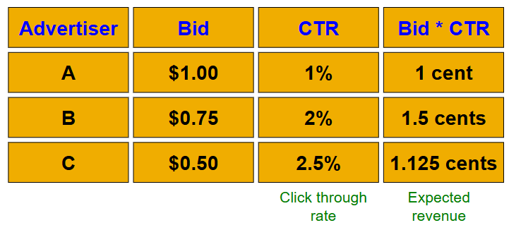
  • so, instead of raw bids, we use “expected revenue per click” (i.e., Bid * CTR)

• the optimal solution is to sort by expected revenue per click, and only show the advertisers at the top

  • unfortunately, this solution isn’t possible since the exact CTR of an ad is unknown, and advertisers have limited budgets and bid on multiple ads. So, we have to use other algorithms instead.

AdWords problem inputs:

1. set of bids by advertisers for search queries

2. CTR for each advertiser-query pair

   • NOTE: we don’t exactly know these values; they’re the search engine’s best estimates based on historical data

3. budget for each advertiser (perhaps for 1 month, or 1 day, etc.)

4. limit on the number of ads to be displayed with each search query

AdWords problem output:

• respond to each search query with a set of advertisers such that:

  1. the size of the set <= limit on the number of ads per query

  2. each advertiser shown has actually bid on the search query

  3. each advertiser shown has enough budget left to pay for the ad if it is clicked upon

What are the two complications with the AdWords problem? Mention exploration and exploitation

1. Budget

   • each advertiser has a limited budget, and the search engine must guarantee that the advertiser will not be charged more than their daily budget

2. CTR of a query-ad pair is unknown (i.e., each ad has a different likelihood of being clicked for a given query)

   • CTR estimate for a given query-ad pair is measured historically, and it’s a very hard problem where we must balance exploration vs exploitation

   • exploit: should we keep showing an ad for which we have good historical estimates of CTR?

   • explore: should we show a brand new ad to get a better sense of its CTR?

Describe the greedy algorithm for the AdWords problem, and its competitive ratio.

Assume a simplified environment.

Suppose the following simplified assumptions:

• there is 1 ad shown for each query

• all advertisers have the same budget B

• all ads are equally likely to be clicked (i.e., equal CTR)

• the value of each ad is the same (=1) (i.e., expected revenue per click = bid * CTR = 1)

The greedy algorithm works as follows:

• for a query, pick any advertiser who has bid 1 for that query

• competitive ratio: ½ 

  • worst case scenario: A bids on query x, B bids on queries x and y, and both have budgets of $4. Assume the query stream is x x x x y y y y. Then, the greedy approach could show ad B 4 times in a row (for query x). Then, it fails to show any ad for query y. Here, the greedy algorithm’s revenue = $4, while the optimal algorithm’s revenue = $8
    

NOTE: the greedy algorithm is deterministic - it always resolves draws in the same way

Describe the BALANCE algorithm for the AdWords problem, and its competitive ratio.

Assume a simplified environment.

Suppose the following simplified assumptions:

• there is 1 ad shown for each query

• all advertisers have the same budget B

• all ads are equally likely to be clicked (i.e., equal CTR)

• the value of each ad is the same (=1) (i.e., expected revenue per click = bid * CTR = 1)

The BALANCE algorithm works as follows:

• for a query, pick the advertiser with the largest unspent budget

• break ties arbitrarily, but in a deterministic way

• competitive ratio for 2 advertisers = ¾ 

• competitive ratio for any number of advertisers = 1-1/e = approx. 0.63

No online algorithm has a better competitive ratio

Describe 3 applications of the market-basket model

The market-basket model consists of a large set of items, and a large set of baskets where each basket is a small subset of items.

Potential applications include:

1. baskets = things one customer bought during one trip to the grocery store, items = things sold in grocery store

2. baskets = sentences, items = documents containing those sentences

   • i.e., basket for sentence x contains all documents d1, d2, … in which sentence x appears

   • items that appear together too often (in the same basket) could represent plagiarism

   • notice items do not have to be “in” baskets; it’s the other way around here (since baskets (sentences) are “in” items (documents)), but typically its better if baskets have a small number of items while items can be in a large number of baskets

3. baskets = patients, items = drugs and side effects

   • used to detect combinations of drugs that result in particular side effects

Describe what frequent itemsets are (in terms of support) in the Market-Basket model.

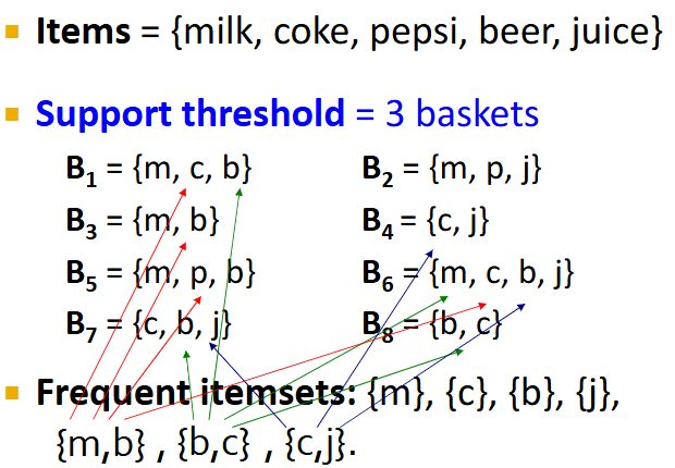
Given a large set of items (things sold in supermarket) and a large set of baskets (each being a small subset of items representing things one customer bought on one trip), we often want to find sets of items that appear together “frequently” in baskets

Given an itemset I, its support is the number of baskets containing all items in I

Given a support threshold s, the sets of items that appear in at least s baskets are called frequent itemsets

Describe what association rules are in the Market-Basket model

Given a large set of items (things sold in supermarket) and a large set of baskets (each being a small subset of items representing things one customer bought on one trip), we often want to discover association rules:
people who bought {x,y,x} tend to buy {v,w}.

Association rules are if-then rules about the contents of baskets:

{i1,i2,…,ik} → j means “if a basket contains items i1, i2, …, ik, then it is ‘likely’ to contain item j”

NOTE: in order to find association rules, we must first find frequent itemsets.

How can we find the support, confidence, and interest of association rules? e.g., find the confidence and interest of rule {m,b} → c

Recall, association rules are structured as {i1, i2,…, ik} → j. In practice, there are many rules, but we only want to find significant/interesting ones.

Support of association rule I → j: support of I = # baskets containing items i1, i2,…, ik

Confidence of association rule I → j: probability of j given I = i1, i2,…, ik

• conf(I → j) = support(IUj) / support(I) = (# baskets containing items i1, i2,…, ik, and j) / (# baskets containing items i1, i2,…, ik)

• output closer to 1 = high confidence

Interest of association rule I → j: difference between its confidence and the fraction of baskets that contain j

• interest(I → j) = conf(I → J) - Pr[j] = (confidence of I → j) - ((# baskets containing item j)/(# baskets))

• output > 0.5 or < -0.5 = high interest

what’s the general process for finding good quality association rules? Mention the hard part, and what we can derive from a rule in terms of set frequency.

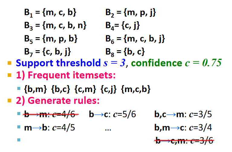
problem/goal: find all association rules with support >= s and confidence >= c

hard part: finding frequent itemsets

• if I = {i1, i2, …, ik} → j has high support and confidence, then both {i1, i2, …, ik} and {i1, i2, …, ik, j} will be “frequent”

procedure for mining association rules:

1. find frequent itemsets I: I₁, I₂, …, I_n

2. generate rules

   • for every subset A of a frequent itemset I_n, generate a rule A → setDiff(I_n, A)

     • since I_n is frequent, so is A

   • compute the rule’s confidence

     • keep in mind that if A→D is below confidence, so is A→CD

     • we can generate “bigger” rules from smaller ones

   • output rules above confidence threshold

describe how data is stored when dealing with finding frequent itemsets, and what the main bottleneck is for frequent-itemset algorithms.

Data is kept in flat files (e.g., csv or txt) stored on disk. It is stored basket-by-basket, where items are positive integers and boundaries between baskets are -1. Baskets are small but we have many baskets and many items.

For each basket, we’re gonna need to find all of its subsets of a particular size. We do this in main memory; to generate all subsets of size k, we use k nested loops. Since baskets are small and k is typically small, this cost is negligible.

So, the true cost of mining this data is the number of disk I/O’s (i.e., how often we move data (baskets) between disk and main memory). In practice, all the algorithms we discuss (for finding frequent itemsets) read the data in passes, where all baskets are read in turn (once per pass). Thus, we ultimately measure the cost of finding frequent itemsets by the number of passes an algorithm takes.

NOTE: number of disk I/O’s = number of passes * number of blocks that we move in and out of disk (can contain multiple baskets if main memory size is sufficient).

Thus, for many frequent-itemset algorithms, main memory size is the critical bottleneck. As we read baskets, we need to count something (e.g., occurrences of pairs). However, this means we must be able to store counts of all possible item pairs in main memory (thus the number of different things we can count is limited). We must keep these counts in main memory since swapping counts in and out of disk is a disaster. e.g., assume each pair’s count takes up 4 bytes, so if we have 100,000 items, then there are 5 billion pairs, which means we need 20 GB in main memory to store all pair counts.

To find frequent itemsets, we need to first generate all possible itemsets, and then count them. So, we always generate all itemsets but only count (keep track) of itemsets that in the end turn out to be frequent.

what size of itemsets is hardest to deal with when finding frequent itemsets?

The hardest problem often turns out to be finding the frequent pairs because frequent pairs are common and the probability of being frequent drops exponentially with size.

• frequent singletons = not too difficult since there aren’t too many items, so we can count them all in main memory pretty easily as we pass through the baskets

• frequent pairs = often too many exist to be able to count in main memory

• frequent triplets = rare, so we can pretty easily count them in main memory

Thus, we concentrate on pairs when discussing frequent-itemset algorithms.

Describe the naive approach to finding frequent pairs. When does it fail?

read file once, counting in main memory the occurrences of each pair:

• from each basket of n items, generate its n(n-1)/2 pairs by two nested loops

this approach fails if (# items)² exceeds main memory

• e.g., if each pair’s count takes up 4 bytes and we have 100,000 items, then there are 5 billion pairs, which means we need 20 GB in main memory to store all pair counts

Describe both approaches of counting pairs in memory, and when each approach is better. What’s the problem with both approaches?

Approach 1: count/store all pairs using a triangular matrix

• only requires 4 bytes per pair, but requires us to store all possible pairs

  • justification: n = total number of items, and we count pairs {i,j} i<j. We also keep pair counts in lexicographic order: {1,2}, {1,3}, … , {1,n}, {2,3}, {2,4}, … , {2,n}, {3,4}, …. So, pair {i,j} is at position (i-1)(n-i/2)+j-i. Total number of unique pairs is n(n-1)/2; total bytes = 2n^2. So, triangular matrix only requires 4 bytes per pair.

Approach 2: keep table of triples [i,j,c] = “count of pair {i,j} is c”

• if integers and item ids are 4 bytes, we need 12 bytes per pair, but we only have to store pairs with count > 0

Therefore, approach 1 stores all possible pairs (4 bytes per pair) while approach 2 only stores pairs that actually occur (12 bytes per pair). Thus, approach 2 beats approach 1 if less than 1/3 of possible pairs actually occur.

The problem with both approaches is that if we have too many items, the pairs can’t fit in memory. So, we need another method.

Describe how the A-Priori algorithm works, and what 2 key ideas it relies on.

A-Priori is a 2-pass approach that limits the need for main memory (i.e., it minimizes what it counts by ignoring impossible candidates). It relies on 2 key ideas:

1. Monotonicity: if an itemset I appears at least s times, so does every subset J of I

2. Contrapositive for pairs: if item i does not appear in s baskets, then no pair including i can appear in s baskets

A-Priori works as follows:

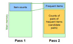
• Pass 1: read baskets and count - in main memory - how often each individual item appears

  • requires memory proportional to # of items

  • NOTE: we’re only interested in whether an item’s count is >= s; thus, we only need to store its count up to s and nothing more beyond that (e.g., if s = 10,000, we only need to keep 2 bytes per count, since a count can only go up to 10,000)

• Pass 2: read baskets from disk again and only count - in main memory - pairs where both items were frequent, ignoring any pair containing an infrequent item; keep only frequent pairs (>=s)

  • requires memory proportional to square of frequent items only (for counts), as well as a list of the frequent items from pass 1 (so we know what must be counted)

    • by additionally storing frequent items, we can read through the items in a basket and ignore any items that aren’t in the list of frequent items; then, for all remaining items, we generate all possible pairs and increment each of their counts

what’s a slight modification we can make to potentially save more space in the A-Priori algorithm?

Recall, we need to store a list of all n frequent items in the second pass.

However, to save more space, we can renumber the n frequent items so the pair counts fit compactly in a triangular matrix.

So, we renumber frequent items 1,2,…n, and keep a lookup table relating these new numbers to the original item numbers. Since we’re now storing 2 numbers for each frequent item, this takes up more memory than what we previously stored (which was just the list of frequent items).

However, now we can use the triangular matrix method to store pair counts instead of the triples-table method. However, this is ONLY beneficial if more than 1/3 possible pairs actually occur; otherwise, the triples-table method actually uses less memory.

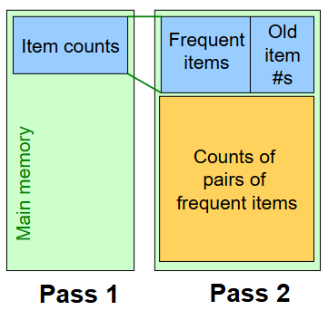
Describe how the general A-Priori algorithm works

For each k, we construct 2 sets of k-tuples (sets of size k):

1. Ck = candidate k-tuples = those that might be frequent sets (support >= s) based on the information from the pass for k-1

   • we must ensure that, for each candidate here, all of their possible subsets of size k-1 are frequent (i.e., exist in Lk-1)

2. Lk = set of truly frequent k-tuples

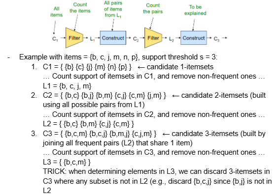
What size k requires the most memory for general A-Priori?

We perform one pass (of reading the dataset) for each k (itemset size), so we need room in main memory to count each candidate k-tuple. Typically, k=2 requires the most memory.

Describe how the PCY algorithm works

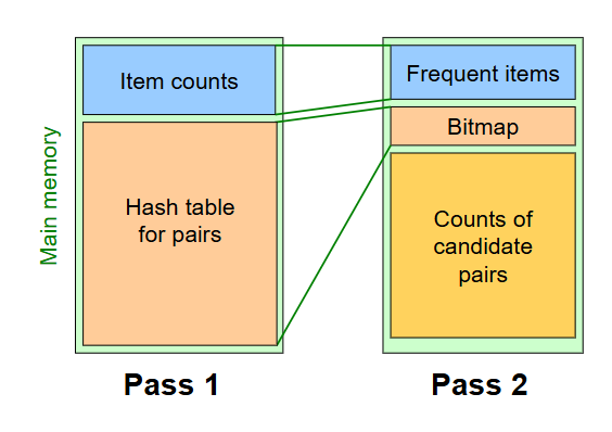
The main problem with A-Priori is that Pass 1 has lots of idle memory, and storing all candidate pair counts in pass 2 needs a huge amount of memory. PCY solves this by reusing idle memory during Pass 1 to help reduce how much we have to count in Pass 1.

Pass 1: 

• read baskets and count - in main memory - how often each individual item appears

• additionally (at the same time), maintain a hash table with as many buckets as fit in memory. For each basket, generate all pairs of items and hash each pair into one of these buckets, incrementing the bucket’s count by 1 each time a pair is hashed into it. 

  • NOTE: for a bucket’s count, we only need to go up to s

  • Observation: if a bucket contains a frequent pair, then the bucket is surely frequent. On the other hand, for a bucket with total count less than s, none of its pairs can be frequent.

Between passes:

• replace buckets by a bit vector, where 1 = frequent bucket (i.e., count >= s) and 0 = infrequent bucket

• since we replaced 4-byte integer counts with bits, the bit vector only requires 1/32 memory (i.e., instead of representing each bucket’s count with a 4-byte integer, we only use 1 bit)

Pass 2:

• read baskets from disk again and only count - in main memory - pairs that meet both conditions:

  1. both items are frequent (>= s)

  2. the pair hashes to a bucket whose bit in the bit vector is 1

• only keep frequent pairs (count >= s)

  • NOTE: both conditions above are necessary for a pair to have a chance of being frequent

Describe the main memory details of PCY, and when it beats A-Priori

• buckets require a few bytes each; # of buckets is O(main memory size)

• on the second pass, a table of (item, item, count) is essential; we CANNOT use a triangular matrix approach

  • why? because pairs that are eliminated because they hash to an infrequent bucket are scattered all over the place and cannot be organized into a nice triangular array

  • thus, the hash table must eliminate approximately 2/3 of candidate pairs for PCY to beat A-Priori

Pass 1:

• space to count each item: typically 4 bytes per item

• rest of the space is used for as large of a hash table as we can, containing a 4-byte counts for each bucket

  • Since each bucket requires 4 bytes, we need to know the number of buckets. Turns out, the # buckets is O(main memory size).

what is bi-partitioning, and what defines a “good” partition of an undirected graph G(V,E)?

• Networks are often organized into modules, clusters, and communities, and our goal is to find densely linked clusters/partitions

• For bi-partitioning, given an undirected graph G(V,E), our task is to divide the vertices into two disjoint groups A, B

• A “good” partition is one where we:

  • Maximize the number of within-group connections (i.e., edges)

  • Minimize the number of between-group connections

How do we express partition quality via cut for undirected and directed graphs?

Cut: set of edges with only one vertex in a group (i.e., sum of weights for all edges with one endpoint in group A and the other in group B)

what’s the minimum cut criterion for partitioning a graph? What’s the problem with it?

• Minimum-cut criterion: minimize weight of connections between groups (i.e., find A and B that minimize cut(A,B); argmin_A,B cut(A,B))

  • Problem: min-cut only considers external cluster connections and does not consider internal cluster connectivity

    • Degenerate cases can occur, where the optimal cut != minimum cut

    • Solution: normalized-cut criterion

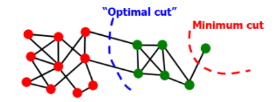
what’s the normalized cut criterion for partitioning a graph? How do we calculate it for weighted and unweighted graphs?

• Normalized-cut criterion: calculates connectivity between groups relative to the density of each group

  • preferred over minimum cut criterion; produces more balanced partitions

• ncut(A,B) = cut(A,B)/vol(A) + cut(A,B)/vol(B)

  • vol(A) = total weight of the edges with at least one endpoint (k) in A = sum of degrees of all nodes in A

    • for weighted graphs, the degree of a node is the sum of the weights of the edges touching it

  • cut(A,B) = total weight of edges Eij where i∈A and j∈B

  • NOTE: lower scores are better; 0.065 identifies 10x better partition than 0.5

Can we actually find the optimal normalized cut for a graph in practice?

Computing the exact optimal (minimum) normalized cut is NP-hard; we can use methods like spectral clustering to relax it and find an approximate solution

Define the following: adjacency matrix, degree matrix, and Laplacian matrix

Matrix representations of graphs:

• Adjacency matrix (A): nxn matrix, where aij = 1 if an edge exists between nodes i and j

  • symmetric since graph is undirected

  • real/orthogonal eigenvectors

• Degree matrix (D): nxn diagonal matrix, where dii = degree of node i (i.e., number of edges connecting to node i)

• Laplacian matrix (L): nxn symmetric matrix, where L = D - A

  • eigenvalues are non-negative real numbers, and eigenvectors are real/orthogonal

  • sum of each row is 0, sum of each col is 0

  • trivial eigenpair: x = (1,...,1)

How do we bi-partition a graph using spectral partitioning?

1. Pre-processing: construct matrix representation of graph

2. Decomposition: compute eigenvalues (λ) and eigenvectors (x) of the matrix, and map each point to a lower-dimensional representation based on one or more eigenvectors (xi)

   • Lx = λx

   • NOTE: each eigenvector xi (i’th column in x) corresponds to the i’th smallest eigenvalue λi; λ1 is the trivial mode (λ1=0)

   • e.g., map points/vertices to lower-dimensional representation based on eigenvector x2, where each node i corresponds to scalar x2[i] for i = 1…6

3. Grouping: assign points to two or more clusters based on the new representation

   • e.g., sort components of the reduced 1d vector (eigenvector x2) and identify clusters by splitting the sorted vector into two (using a split of 0): nodes 1,2,3 -> cluster A, nodes 4,5,6 -> cluster B

   • NOTE: splitting at 0 or the median value are naive approaches; there are more expensive approaches not covered in this course

How do we perform K-way spectral clustering to partition a graph into k non-overlapping clusters/communities?

• Approach 1: recursive bi-partitioning

  • recursively apply bi-partitioning algorithm in a hierarchical divisive manner

  • inefficient and unstable

• Approach 2 (better): cluster multiple eigenvectors

  • build a reduced space from multiple eigenvectors

  • i.e., the idea is that we describe each point/node by multiple eigenvectors (e.g., point p = values from eigenvectors corresponding to 1st - 3rd smallest eigenvalues = (x1[p], x2[p], x3[p])), and then run k-means clustering on the resultant 3-dimensional point representations

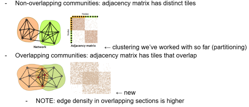
What’s the purpose for overlapping communities and how can we differentiate between non-overlapping and overlapping communities in an adjacency matrix?

In cases like Facebook relationships (where nodes = Facebook users, edges = friendships), many social communities exist and overlap with each other (e.g., same work, same high school, same math class, same basketball team); for examples like this, it makes sense for clusters/communities to overlap instead of being separate.

Non-overlapping communities: adjacency matrix has distinct tiles

• this is the type of clustering we’ve worked with so far (partitioning)

Overlapping communities: adjacency matrix has tiles that overlap

• edge density in overlapping sections is higher

What is the goal of AGM (Community-Affiliation Graph Model)?

goal: define a model that can generate networks

• the model will have a set of parameters that we need to estimate using our data, and these estimates will implicitly detect communities

i.e.,

• key question: given a set of nodes, how do communities “generate” edges of the network? 

• solution: use AGM (which is a generative model) to generate the network’s edges

Given an AGM (which is a generative model), how do we produce a network step-by-step?

AGM is a generative model B(V,C,M, {pc}) for graphs, where:

• V = nodes (same as nodes in our network)

• C = communities (same as clusters in our network)

• M = memberships (connections of nodes to communities)

• Pc = probability of community c

Given an AGM, we generate the network’s edges as follows:

• For each pair of nodes u,v in community c, we connect them with probability Pc

  • overall edge probability = P(u,v) = 1 - [product of cEM_u M_v](1-p_c) = 1 - [product of (1-Pc) for each community c that BOTH u and v belong to], where Mu = set of communities node u belongs to

    • if u,v share no communities, P(u,v) = 0

    • i.e., think of it as an OR function: if at least one community says YES, we create an edge

• Once we have P(u,v), simply flip a coin with this probability to decide whether to connect an edge between these nodes or not; repeat this for all node pairs

What types of community structures can be expressed by an AGM?

AGM is very flexible; it can express a variety of community structures such as non-overlapping, overlapping, nested, etc.

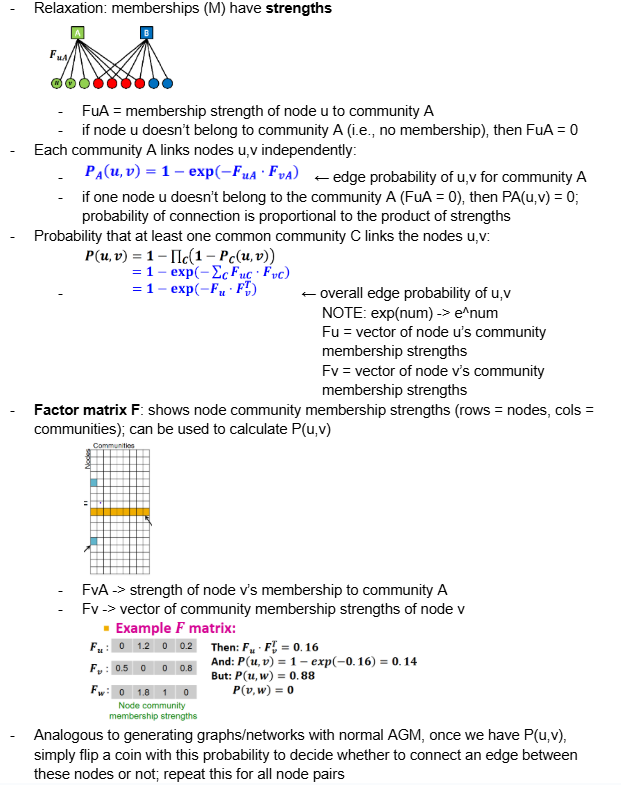
Explain how we can generate a network given a relaxed AGM, where memberships (M) have strengths

see pic: describes how to calculate edge probability for each pair of nodes, which we use to generate the final network.

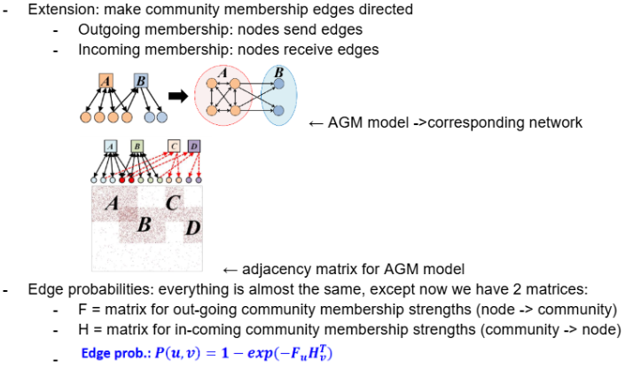
Explain how we can generate a network given a directed AGM, where community membership edges are directed

Recall, the Factor matrix F shows node community membership strengths (rows = nodes, cols = communities); can be used to calculate P(u,v)

• FvA -> strength of node v’s membership to community A

• Fv -> vector of community membership strengths of node v

However, now when calculating edge probabilities we use 2 matrices:

• F = FuA → community membership strength of outgoing edge from node u to community A

• H = HvA → community membership strength of incoming edge from community A to node v

The probability of generating a directed edge from u to v is 1 - exp(-Fu Hv^t)

What is the goal of trawling?

• Goal: detect small, dense communities in web graphs that are highly interconnected (e.g., people that are all talking about the same set of things/topics)

• Intuition: a community on the web can be modeled as a dense bipartite subgraph, where:

  • left side (X) = people or sources (bloggers, users, authors)

  • right side (Y) = objects or targets (webpages, topics, papers)

how do we define small, dense communities in highly interconnected web graphs?

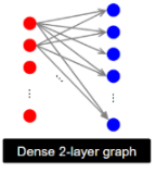
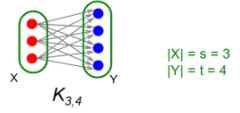
We produce a complete (i.e., fully connected) bipartite subgraph K_s,t

• s nodes on the left, each linking to exactly the same t other nodes on the right

• i.e., K_s,t is a fully connected subgraph with s nodes on one side, each connected to t nodes on the other side

i.e., Given a frequency threshold f, we want to define Ks,t, where we have s nodes (each node si is represented as a set Si, where Si’s elements are the nodes that node si connects to), and a set of t nodes (for which all t nodes exist in each Si). In plain english, Ks,t = a set of s nodes, each with edges connecting to the same set of t nodes. 

What’s the connection between frequent itemsets in market basket analysis and complete bipartite graphs K_s,t?

• Setting:

  • Market = Universe U of n items

  • Baskets = m subsets of U: S1, S2, …, Sm, where Si is a set of items one person bought

  • Support = frequency threshold f

• Goal: find all subsets T such that T is a subset of Si for at least f sets of Si’s (i.e., items in T were bought together at least f times)

  • For a given webgraph, we want to find all possible/existing bipartite subgraphs Ks,t; these indicate frequent itemsets

• Connection: frequent itemsets (groups of items that appear together in many baskets) = complete bipartite graphs

Given baskets, how do we produce a complete bipartite graph for a frequent itemset?

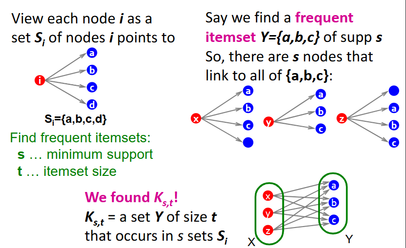
• represent each node i as a set Si of nodes that i points to

• given a minimum support (s) and itemset size (t), look for all sets Y (frequent itemsets) of size t that occur in s sets Si

  • each of these represents a complete bipartite graph K_s,t

• for example, assume we find a frequent itemset Y={a,b,c}, meaning there are s nodes (x,y,z) that link to all of {a,b,c}

  • from here, we can define K_s,t = set Y of size t that occurs in s sets Si, where nodes x,y,z on the left connect to all of nodes a,b,c on the right

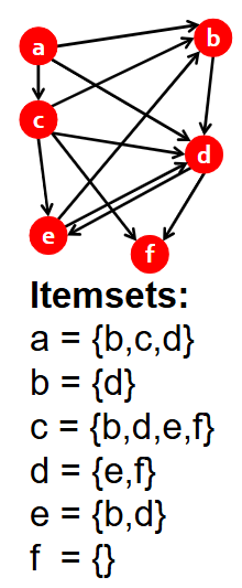
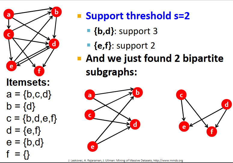
For this graph, find all frequent itemsets and corresponding complete bipartite subgraphs, assuming s=2

What is the purpose of clustering?

• Given a cloud of data points (with a notion of distance between them), we can understand its structure by grouping them into clusters

  • members of a cluster = similar/close to each other

  • members of different clusters = dissimilar

  • members of no cluster = outliers

• Usually, points are in a high-dimensional space (i.e., many features), and distance is measured using a method like Euclidian, Cosine, Jaccard, etc.

What are the 2 methods of clustering?

• Hierarchical:

  • Agglomerative (bottom up): each point starts as a cluster and we repeatedly combine the two nearest clusters into one

  • Divisive (top down): start with one cluster and recursively split it

Point assignment: maintain a set of clusters and points belong to the nearest cluster (e.g., K-means)

What are the 3 key questions for hierarchical agglomerative clustering methods?

Remember, the key operation for hierarchical agglomerative clustering is to repeatedly combine two nearest clusters. So, we have three important questions:

1. How do you represent a cluster of more than one point? (i.e., how do you represent the “location” of each cluster to tell which pair of clusters is closest?)

2. How do you determine the nearness of clusters?

3. When to stop combining clusters?

Provide the answer to the first key question for hierarchical agglomerative clustering methods:

1. How do you represent a cluster of more than one point? (i.e., how do you represent the “location” of each cluster to tell which pair of clusters is closest?)

Solution: represent each cluster by its centroid (e.g., for Euclidean, each cluster’s centroid is the average of its data points)

Solution (Non-Euclidean): when we can’t use the “average” of points but rather the points themselves, we represent each cluster by its clustroid (the data point closest to other points (e.g., smallest sum of squares distances to other points))

Provide the answer to the second key question for hierarchical agglomerative clustering methods:

2. How do you determine the nearness of clusters?

• Solution: measure cluster distances by distances of centroids

• Solution (Non-Euclidean): treat clustroid as if it were the centroid

Provide the answer to the third key question for hierarchical agglomerative clustering methods:

3. When to stop combining clusters?

• Approach 1: predefined k, stop when we have k clusters (makes sense when we know the data naturally falls into k classes)

• Approach 2: stop when the next merge would create a cluster with low cohesion (i.e., a bad cluster)

  • cohesion could be defined as:

    • (1) the diameter of the merged cluster = maximum distance between points in the cluster

    • (2) radius = maximum distance (or average distance) of a point from the centroid or clustroid

    • (3) density-based approach = diameter (or average distance) divided by number of points in the cluster

What’s the naive implementation of hierarchial clustering, and what’s the performance?

• Naive implementation: compute pairwise distances between all pairs of clusters, then merge 

  • Performance: O(N^3),

  • However, careful implementation using priority queue can reduce it to O(N^2 log(N))

    • Still too expensive for really big datasets that do not fit in memory

Describe how the K-means clustering algorithm works, step-by-step

NOTEL this algorithm assumes Euclidean distance (see formula in pic) for n dimensions and points p, q:

1. Pick k (number of clusters)

2. Initialize clusters by picking one point per cluster

• Approach 1: sampling

  • cluster a sample of the data (fitting in main memory) using hierarchical clustering to obtain k clusters

  • pick a point from each cluster (e.g., point closest to centroid)

• Approach 2: picking dispersed set of points

  • pick first point at random

  • pick the next point to be the one whose minimum distance from the selected points is as large as possible

  • repeat until you have k points

3. For each remaining point, place it in the cluster whose current centroid is the nearest

4. After all points are assigned, update the locations of centroids of the k clusters

5. Reassign all points to the closest centroid (points may move between clusters)

6. Repeat 4 and 5 until convergence (i.e., until points don’t move between clusters and centroids stabilize)

What’s the optimal way to select k for k-means clustering?

• How to select k: 

  • Try different k, looking at changes in average distance to centroid as k increases

  • Optimal k occurs when average falls rapidly, followed by little change

What’s the time complexity of k-means clustering; how can we improve this performance?

• In each round, we have to examine each input point exactly once to find closest centroid

• Each round is O(kN) for N points, k clusters

• Issue: number of rounds to convergence can be very large 

  • Solution: cluster in a single pass over the data using the BFR algorithm

what is the BFR algorithm’s purpose?

BFR algorithm: extension of k-means to large data

• Variant of k-means designed to handle very large datasets stored in disk

• Efficient way to summarize clusters (want memory required O(clusters) and not O(data))

What’s the key assumption made by the BFR algorithm? Because of this, what shape are the clusters?

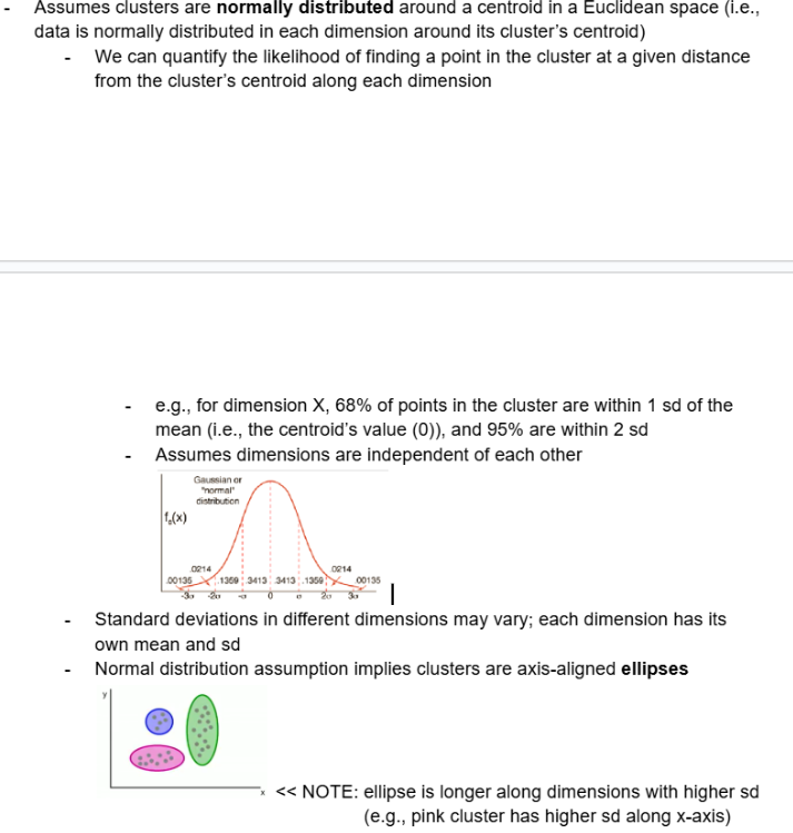
• Assumes clusters are normally distributed around a centroid in a Euclidean space (i.e., data is normally distributed in each dimension around its cluster’s centroid)

  • We can quantify the likelihood of finding a point in the cluster at a given distance from the cluster’s centroid along each dimension

    • e.g., for dimension X, 68% of points in the cluster are within 1 sd of the mean (i.e., the centroid’s value (0)), and 95% are within 2 sd

    • Assumes dimensions are independent of each other

• Standard deviations in different dimensions may vary; each dimension has its own mean and sd

• Normal distribution assumption implies clusters are axis-aligned ellipses

  • NOTE: ellipse is longer along dimensions with higher sd

Describe the BFR algorithm in-depth

1. start with first load in-memory and select k initial centroids using any main memory clustering algorithm

2. assign points to DS

3. assign remaining points to CS, RS

4. summarize all clusters in DS and CS, store summary statistics (N, SUM, SUMSQ) in main memory, discard DS and CS points

   1. each cluster is fully represented by its summary statistics

5. store RS points in main memory

6. load next set of data in-memory (including previous RS points and DS/CS statistics)

7. add points that are sufficiently close to a DS cluster centroid into the DS

8. adjust statistics of the DS clusters to account for the new points

   1. incrementing N, SUM, and SUMSQ is easy and not computationally complex

9. discard DS points

10. for all remaining points, run main memory clustering algorithm to assign them to CS clusters

11. store new CS cluster statistics, adding all unassigned points to the RS

12. discard CS points, store RS points in main memory

13. consider merging any new/existing CS clusters into one (based on variance)

14. repeat 6-13 until final round; in final round, merge all CS clusters into one and all RS points into their nearest DS or CS cluster

Detailed algorithm:

• Algorithm:

  • At any given time, main memory contains (1) current set of points read from disk, (2) metadata of clusters from previously read points

• Points are read from disk one main memory-full at a time

• Most points from previous memory loads are summarized by simple statistics

• To begin, from the initial load, we select the initial k centroids by some sensible approach:

1. Take k random points

2. Take a small random sample

3. Cluster optimally (e.g., pick a random sample point, and then k-1 more points, each as far from the previously selected points as possible)

• Keep track of 3 classes of points:

  • Discard Set (DS): points close enough to a centroid to be summarized (points in blue ellipse)

  • Compression Set (CS): groups of points that are close together but not close to any existing centroid (points in yellow ellipses)

    • these points are summarized, but not assigned to a cluster

  • Retained Set (RS): isolated points waiting to be assigned to a compression set (orange dots)

    • we have to keep track of these points in memory (unlike points in the DS and CS, which we throw away and only keep metadata for)

• Summarize sets of points:

  • For each cluster, the Discard Set (DS) is summarized by:

    • (1) integer N, representing the number of points in the cluster

    • (2) vector SUM, whose i’th component is the sum of the coordinates of the points in dimension i

    • (3) vector SUMSQ, whose i’th component is the sum of squares of the coordinates of the points in dimension i

    • Comments: 

      • 2d+1 values represent a cluster of any size, where d = number of dimensions 

        • why? len(N)+len(SUM)+len(SUMSQ) = 1+d+d = 1+2d

      • SUMi / N = average in each dimension (i.e., the centroid), where SUMi = i’th component of SUM

      • (SUMSQi / N) - (SUMi / N)^2 = variance of a cluster’s discard set in dimension i, where SUMSQi = i’th component of SUMSQ

        • sd = sqrt(var)

• Process the memory-load of points:

1. Find points that are sufficiently close to a cluster centroid and add those points to that cluster and the DS

• adjust statistics of the clusters to account for the new points: N, SUM, SUMSQ

• these points are summarized and then discarded

• how do we decide if a point is close enough to a cluster? BFR suggestion is to take points with a Mahalanobis distance (likelihood of point belonging to a centroid) less than a threshold (i.e., take points with a high likelihood of belonging to the currently nearest centroid (fulfilling normal distribution))

2. Use any main memory clustering algorithm to cluster the remaining points and the old RS

• clusters go to the CS, outlying points to the RS

3. Consider merging compressed sets in the CS

• how do we decide whether two compressed sets (CS) deserve to be combined into one? BFR suggestion is to compute the variance of the combined subcluster (N, SUM, and SUMSQ allow us to calculate this quickly), and combine if the combined variance is below some threshold

4. If this is the last round, merge all compressed sets in the CS and all RS points into their nearest cluster

What’s the issue with BFR and k-means, and what’s the solution?

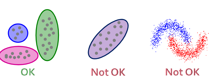
• Issue: BFR/k-means assumes clusters are normally distributed in each dimension, and - since axes are fixed - ellipses at an angle are NOT ok

• Solution: CURE (Clustering Using REpresentatives) algorithm

What does the CURE algorithm assume? What shape does it allow clusters to be, and how are clusters represented?

CURE algorithm: extension of k-means to clusters of arbitrary shapes

• Assumes a Euclidean distance (i.e., between any two points, we can always find the midpoint by taking the average)

• Allows clusters to assume any shape

• Uses a collection of representative points to represent clusters

  • Unlike BFR/k-means, which use one point to represent a cluster

How does the CURE algorithm work?

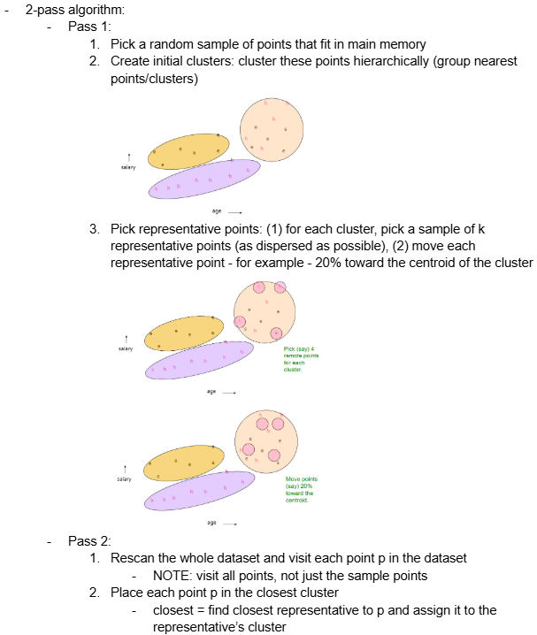
2-pass algorithm:

• Pass 1:

  1. Pick a random sample of points that fit in main memory

  2. Create initial clusters: cluster these points hierarchically (group nearest points/clusters)

  3. Pick representative points: (1) for each cluster, pick a sample of k representative points (as dispersed as possible), (2) move each representative point - for example - 20% toward the centroid of the cluster

• Pass 2:

  1. Rescan the whole dataset and visit each point p in the dataset

     • NOTE: visit all points, not just the sample points

  2. Place each point p in the closest cluster

     • closest = find closest representative to p and assign it to the representative’s cluster

What’s the performance of the CURE algorithm?

Performance: O(N); one pass of data (I think??? not sure)