SOCIAL SCIENCE Q2

Summary

Demand

Quantity of a good or service that consumers are willing and able to purchase.

Law of Demand

Price increase, Quantity demanded decreases, assuming ceteris paribus

Demand Schedule

Table showing Qd at different prices

Demand Curve

Graphical representation of the demand schedule

Demand Function

Qd = a - bP

Factors affecting demand (shift)

• Price of the Good

• Income of Consumers

• Prices of Related Goods

• Tastes and Preferences

• Expectations

Supply

Quantity of a good or service that producers are willing and able to sell

Law of Supply

As price increases, quantity supplied also increases, assuming ceteris paribus

Supply Schedule

Table showing Qs at different prices

Supply Curve

Graphical representation of Supply schedule

Supply Function

Qs = a - bP

Factors affecting supply (shift)

• Input prices

• Technology

• Taxes and Subsidies

• Number of Sellers

• Price Expectations

Market Equilibrium

Point where Qd = Qs

Surplus (Excess Supply)

Occurs when price is set above equilibrium price

Qs > Qd

Shortage (Excess Demand)

Occurs when price is set below equilibrium price

Qd > Qs

Government interventions

Price Ceilings

Price Floor

Price Ceiling

• Maximum legal price that sellers can charge

• Set below equilibrium

• Leads to shortage

Price Floor

• Minimum legal price that sellers must charge

• Set above equilibrium

• Leads to surplus

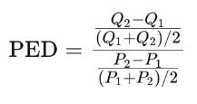
Price Elasticity of Demand (PED)

Measures how much Qd responds to change in price

Elastic Demand

• There are more available substitutes

• Consumers react strongly to price changes

• E_p > 1

Inelastic Demand

• Price change cause only small change in quantity

• E_p < 1

Perfectly Inelastic

• People buy the same amount no matter the price

• E_p = 0

Unit Elastic

• The percentage change in price equals the change in demand

• E_p = 0

Perfectly Elastic

• Tiny price increase makes demand drop to zero

• E_p = infinity

Factors Affecting Price Elasticity of Demand

• Availability to Substitutes

• Necessity vs. Luxury

• Proportion of Income

• Time Period

Total Revenue and Elasticity

TR = P x Qty

TR | Elastic Demand

Price decrease = TR increases

TR | Inelastic Demand

Price increase = TR increase

TR | Unit Elastic

Changes in price do not affect TR

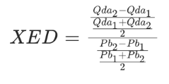
Cross Price Elasticity of Demand (XED)

Measures the responsiveness of Qd of one good to a change in the price of the other good

Goods are non-related

= 0

Goods are Substitutes

> 0 | positive

Goods are Complements

< 0 | negative

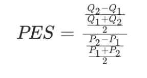
Price Elasticity of Supply (PES)

Measures how much Qs changes when price changes

Focuses on how suppliers respond to changes in price

Unit Elastic

= 1

Elastic

> 1

Inelastic

< 1

Perfectly Elastic

= infinity

Perfectly Inelastic

= 0

Income Elasticity of Demand (YED)

Measures how quantity demanded responds to changes in consumer income

Normal Luxury

> 1

Normal Necessity

0 < E_y < 1

Inferior Goods

< 0

Theory of Choice | Consumer Theory

Interaction of preferences and constraints that guide purchasing decisions

Utility

The satisfaction or pleasure derived from economic activity or consuming goods and services

Total Utility

Overall satisfaction from consuming a specified qty

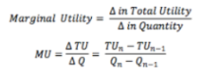
Marginal Utility

The additional satisfaction (increment) received from consuming an extra unti of a good

Law of Diminishing Marginal Utility

As the amount of a good consumed increases, MU decreases

Saturation Point

MU = 0

Maximum point of consumer satisfaction

Production Theory

Transforming production inputs into goods or services Sh

Short-run

At least one production input is fixed

Long-run

All production inputs are fixed

Total Product

Total amount of output produced

Marginal Product

Additional product per unit of labor hired

Average Product

Describes the average productivity of each worker

AP = TP/L

Law of Diminishing Marginal Returns

Adding additional units of a variable input while holding other inputs fixed, a firm eventually gets less and less extra output

Cost

All the opportunity costs in production

Total costs = explicit + implicit costs

Explicit Costs

Input costs that involve a direct disbursement of money

Implicit Costs

Input costs that do not require a disbursement of money

Economic Profit

TR - implict + explicit costs

Cost Components

• Total Costs

• Fixed Costs

• Variable Costs

Fixed Costs

Expenses paid even at zero output

Variable Costs

Expenditures that depend on output

Total Cost

FC + VC

Marginal Costs

Additional cost incurred when producing a extra unit of output

Average Costs

Used to estimate profits by comparing price to cost

Curve is U shaped

MC and AC/AVC relationship

MC curve intersects AC and AVC at their lower points

MC > AC ; MC is falling

MC < AC; MC is rising

Total Revenue

measures qty sold by the price per unit

Marginal Revenue

The change in total revenue resulting from a one-unit change in output

Maximization

TR reaches max point when MR = 0

Profit

Financial gain when TR > TC

Normal Profit

Economic profit is zero

Break Even Point (BEP)

TR = TC; resulting in zero profits

Market Structures

Differentiated based on

• Number of Sellers

• Barriers to Entry

• Price Control

• Product Differentiation

Market Structure Types

• Pure Competition

• Monopolistic Competition

• Oligopoly

• Monopoly

Pure Competition

No. of sellers: No limit
Barriers to Entry: None

Price Control: No price controls

Product Differentiation: Products are identical

Monopolistic competition

No. of sellers: Many buyers and sellers
Barriers to Entry: Few to none

Price Control: Some Control

Product Differentiation: Products are identical

Oligopoly

No. of sellers: Few
Barriers to Entry: High

Price Control: High

Product Differentiation: Can be differentiated or identical

Monopoly

No. of sellers: Only one
Barriers to Entry: High

Price Control: High

Product Differentiation: No product differentiation