Stats Textbook Terms

Cases

Objects described in a set of data. Ex: customers, companies, study subjects, units

Label

Special variable distinguished in different cases

Variable

Characteristics of a case

Values

Different cases have different values

Categorical variable

Places a case into several groups or categories

Quantitative Variable

takes numerical variables for which arithmetic operations such as adding and averaging make sense

key characteristics of data set

who what and why

Explanatory Data Analysis

Examine data and describe their main features

Distribution of a categorical variable

Lists the categories and gives either the count or the percent (or proportion) of the cases that fall in each category

mean x̅

x1+x2+…./n

median M

(n+1)/2 (to find location of median)

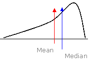
Median versus mean

Median is more resistant to the mean

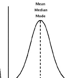
If shape is symmetric, median = mean

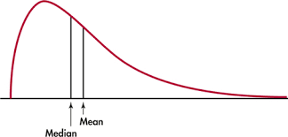
Shape

Skewed where the tail is

Quartiles

25%, 50%, 75%

IQR (Interquartile range)

Q3-Q1

Outlier IQR

1.5 x IQR

Q1- (1.5 x IQR) = lower bound

Q3 + (1.5 x IQR) = upper bound

S (Standard Deviation) Formula

√[ Σ(xi - x̄)² / (n-1) ]

S² (Variance) Formula

∑ (xi - x̄)² / (n - 1)

Degrees of Freedom formula

n-1

What does s measure?

spread about the mean

s=0

No spread

When are variables associated?

If knowing the valuable of one tells you something about the values of the other

Responsive Variable

Measures an outcome of a study

Explanatory Variable

Explains or causes changes in the response variable

Independent Variable

the factor that a researcher manipulates or changes to see how it affects another variable

Dependent Variable

a variable (often denoted by y ) whose value depends on that of another.

Scatterplot

Shows the relationship between two quantitative variables measured on the same cases

Positively Associated

two things are positively associated when above-average values of one tend to accompany above-average values of the other and below-average values tend to occur together

Negatively Associated

Two variables are negatively associated when above-average values of one tend to accompany below-average values of the other, and vice versa

Correlation (r ) formula

Causation

x → y

Common Response

z→x and y

Confounding

x→ y

z→ y

Sample Space S

The set of all possible outcomes

Event

An outcome or a set of outcomes of a random phenomenon. Subset of the sample space

ex: exactly four heads

Probability rules

Rule 1. The probability P(A) of any event A satisfies 0 ≤ P(A) ≤ 1.

Rule 2. If S is the sample space in a probability model, then P(S) = 1.

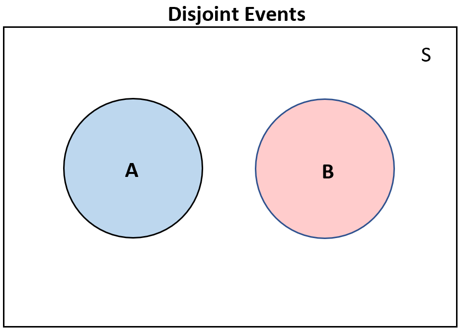
Rule 3. Two events A and B are disjoint if they have no outcomes in common and so can never occur together. If A and B are disjoint,

• P (A or B) = P (A) + P (B)

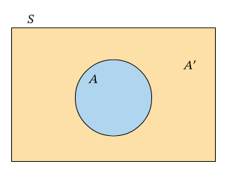
Rule 4. The complement of any event A is the event that A does not occur, written as Ac. The complement rule states that

P (Ac) = 1 − P (A)

Rule 5. Two events A and B are independent if knowing that one occurs does not change the probability that the other occurs. If A and B are independent,

P (A and B) = P (A) P (B)

Disjoint events

Complement A^c

Multiplication rule for independent events

P (A and B) = P (A) P (B)

Independent in probability

The outcome of one event is not influenced by the outcome of another event

Additional Rule

If A and B are disjoint events, then

P (A or B) = P (A) + P (B)

Complement Rule

For any event A,

P (Ac) = 1 − P(A)

RULE FOR UNIONS OF TWO EVENTS

any two events A and B,

P (A or B) = P (A) + P(B) − P (A and B)

Conditional Probability

When P(A) > 0, the conditional probability of B given A is

P(B|A)= P(AandB)/ P(A)

Intersection of events

When P(A) > 0, the conditional probability of B given A is

P(B|A)= P(AandB) P(A)

Independent Events

Two events A and B that both have positive probability are independent if P(B|A) = P(B)

Density Curve

A density curve is a curve that

• Is always on or above the horizontal axis.

• Has area exactly 1 underneath it.

A density curve describes the overall pattern of a distribution. The area under the curve and above any range of values is the proportion of all observations that fall in that range.

symmetric normal density, right skewed/left skewed

Normal distribution density curve

Right skewed density curve

Left skewed density curve

What does the standard deviation control in a curve

the spread of the curve

The 68-95-99.7 Rule

In the Normal distribution with mean μ and standard deviation σ:

Approximately 68% of the observations fall within σ of the mean μ. Approximately 95% of the observations fall within 2σ of μ. Approximately 99.7% of the observations fall within 3σ of μ.

N(μ, σ)

mean μ and standard deviation σ

z score

z = x–μ / σ

Random Variable

a variable whose value is a numerical outcome of a random process.