3.3 Revenues, costs, and profits

Revise this BEFORE 3.3 Business objectives

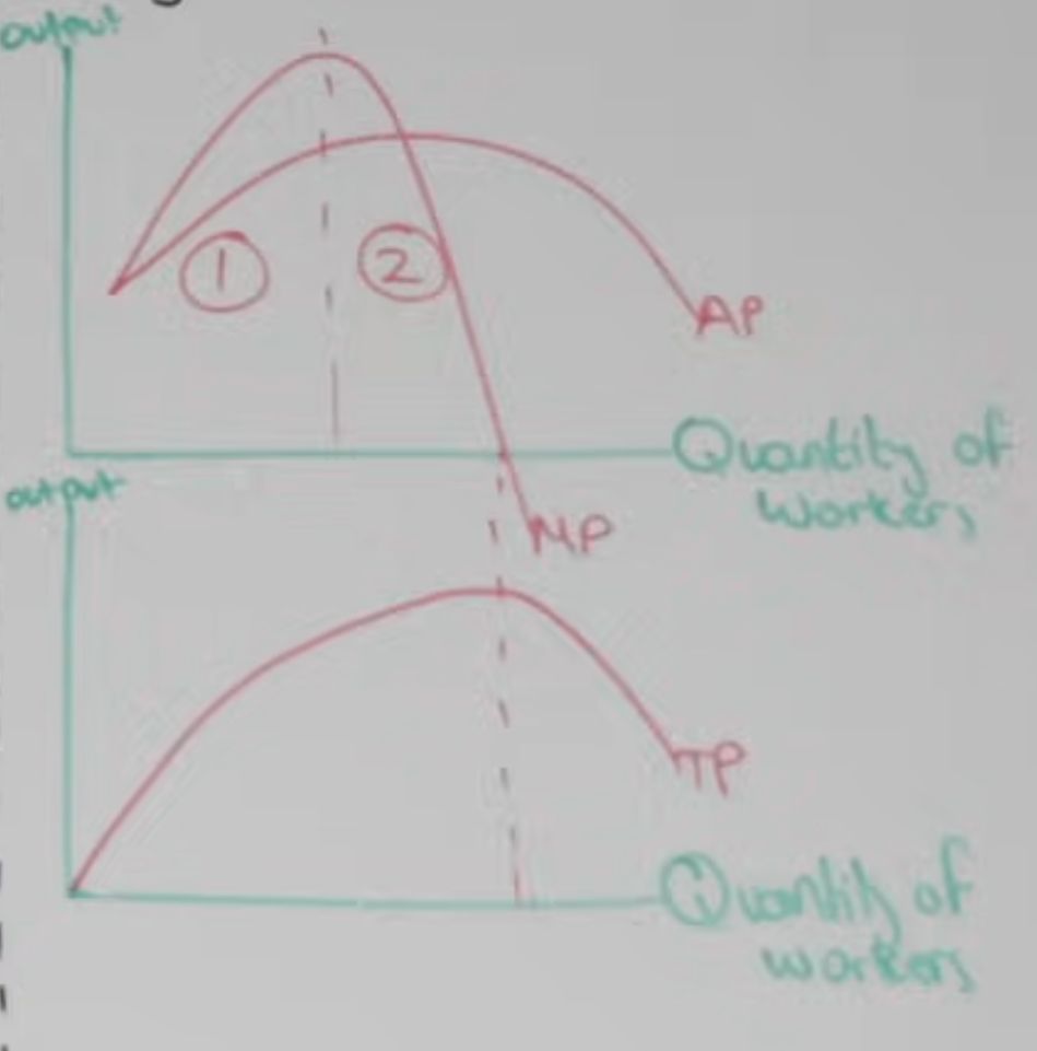
Law of diminishing marginal returns

In the SR when variable factors of production(labour) are added to a stock of fixed factors of production, total/ marginal product (output) will initially rise and then fall.

1. Rises at first due to specialisation+underutilisation of FoP→higher labour productivity→more output

2. Falls afterwards due to limited land + capital(FoP) which become a constrain on production→lower productivity→less output

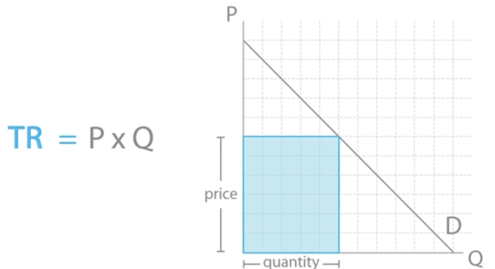
Total revenue

Total money made by sales by a business.

price x quantity sold

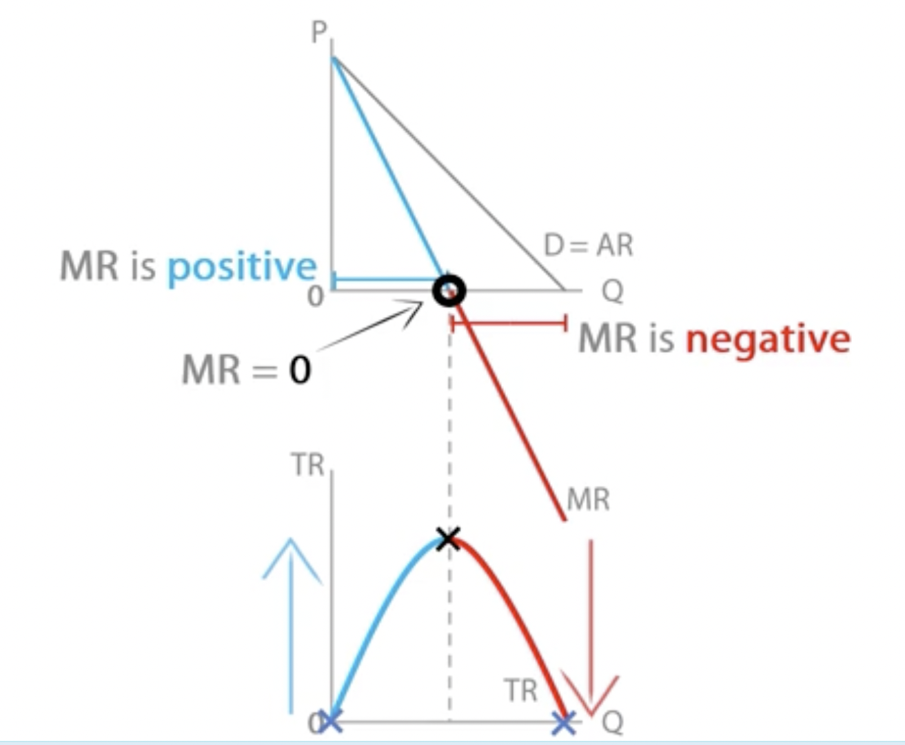
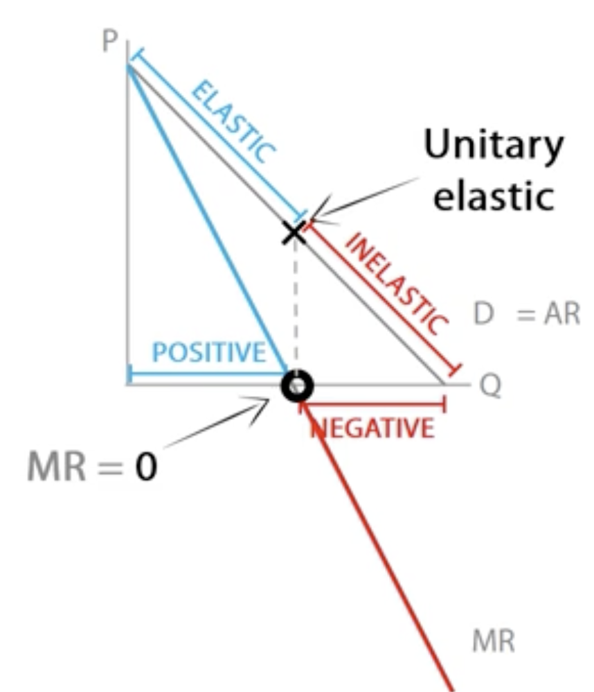
TR reaches its peak when MR = 0.

Average revenue

What a business receives on average from each sale it makes.

AR = total revenue / quantity

AR = price

AR curve = demand curve

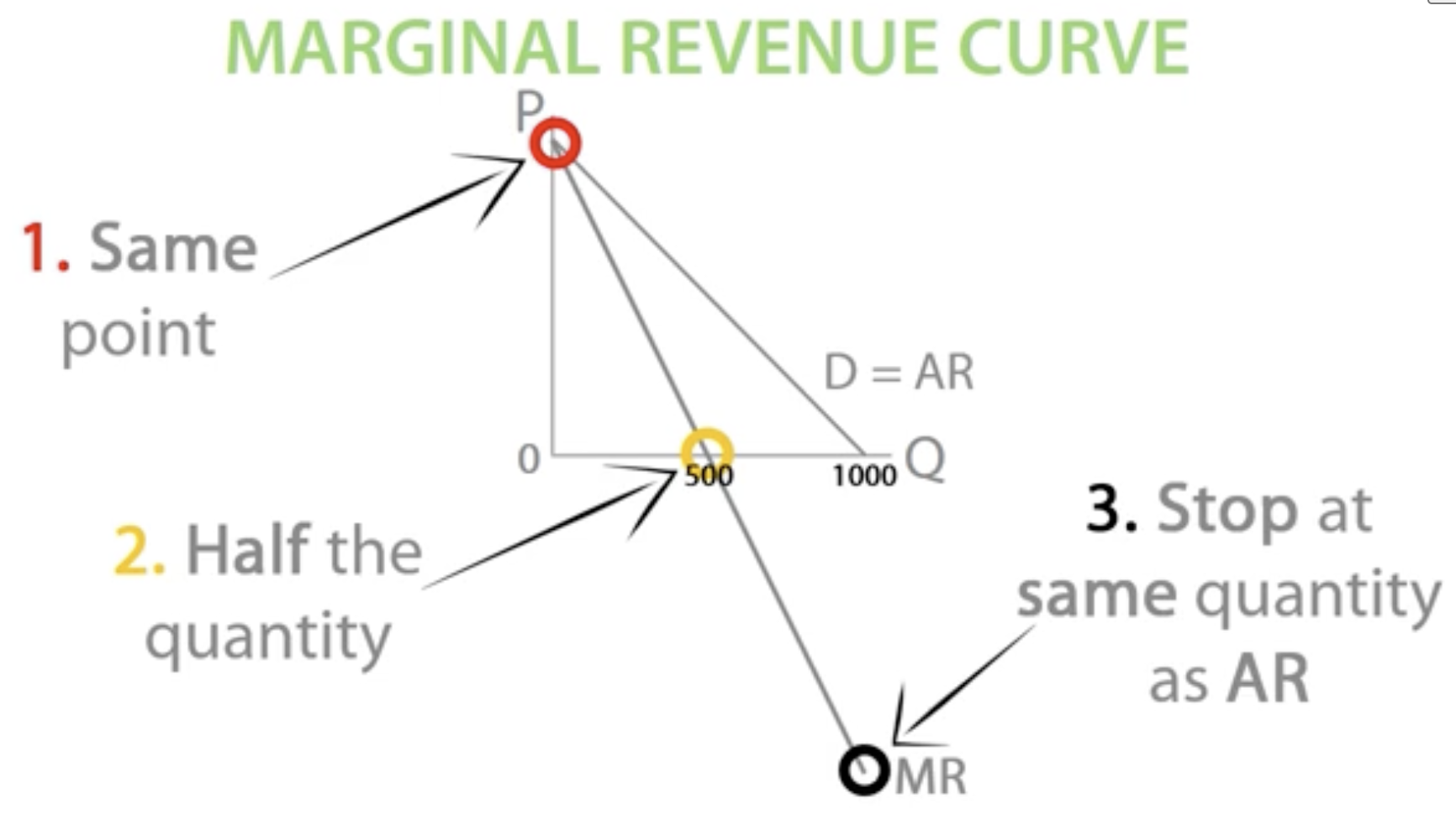
Marginal revenue

Additional revenue a firm makes selling one extra unit of output.

change in TR / change in quantity

Revenue diagram- price takers (perfect competition)

Revenue diagram- price makers

TR is maximised when MR=0, as when MR is positive, TR increases with quantity.

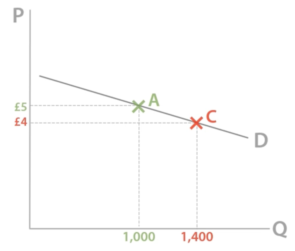
TR and price elasticity of demand

When price ↓ by a small %, quantity demanded ↑ by a larger %, increasing TR overall.

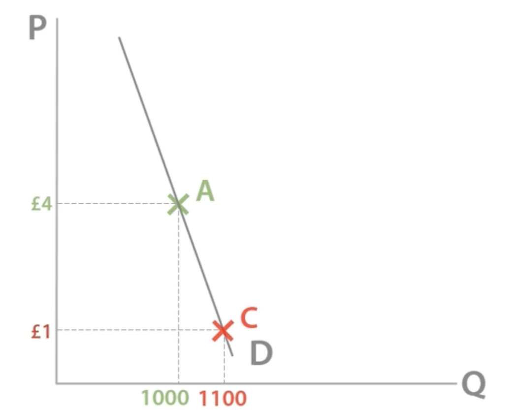
TR and price inelasticity of demand

When price ↓ by a larger %, quantity demanded ↑ by a small %, decreasing TR.

How does PED change along the demand curve

When price is low, a % change in price will have a small effect, so consumers will be unresponsive and demand will be inelastic.

Fixed + variable costs

Variable costs: costs vary with output

e.g. wages, raw material costs, utility bills

Fixed costs: costs that don’t vary with output

e.g. salaries, rent, interest on loans

In the LR, all factors become variable, so there are only variable costs.

• In the SR, one factor must be fixed, so there are only fixed costs.

Total fixed cost (TFC)

TC-TVC or AFC x Q

Have nothing to do with law of diminishing marginal returns.

Average fixed cost (AFC)

TFC/ Q or AC-AVC

Decreases as TFC stays same while Q increases.

Have nothing to do with law of diminishing marginal returns.

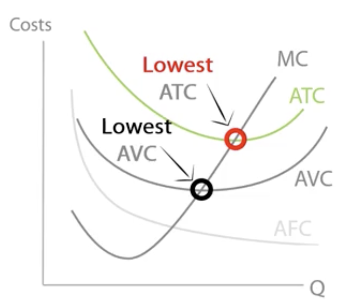
Average variable cost (AVC)

TVC/ Q or AC-AFC

As you employ more workers, productivity increases, ↓AVC, then decreases as output decreases, ↑ AVC.

Average cost (AC) or ATC

TC/ Q or AFC+AVC

Marginal cost (MC)

∆TC/ ∆Q

The extra cost of producing one more unit of output.

-as labour productivity ↑, MP ↑, MC ↓ due to the higher productivity.

-as labour productivity ↓, MP ↓ and MC ↑ due to the lower productivity.

Average total cost/ average cost

TC / Q or AVC + AFC

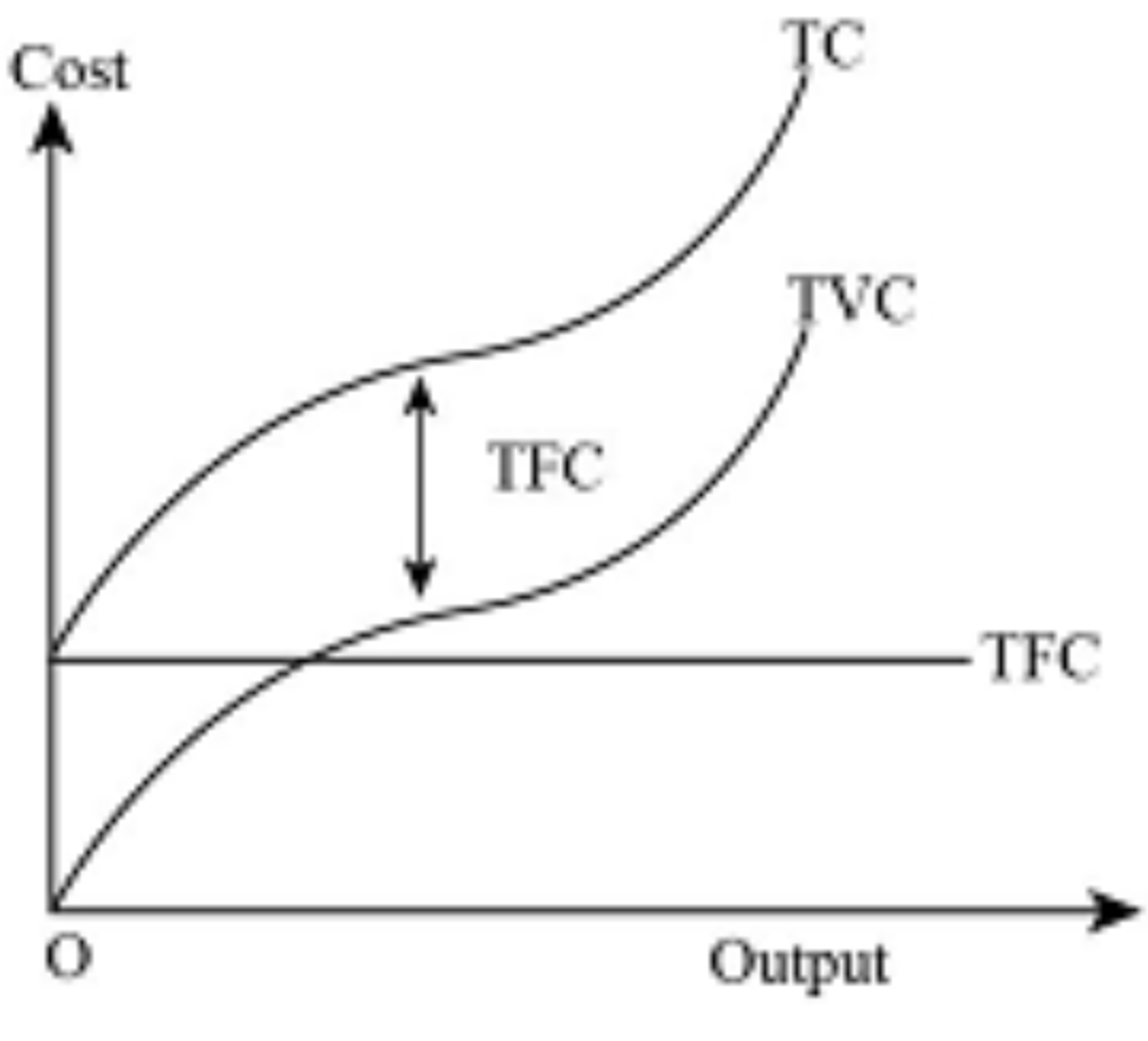
TC,TVC,TFC diagram

TVC rises due to wages paid to workers being employed, slows down as they specialise in their roles so output increases greater than cost, then increases again due to law of diminishing returns.

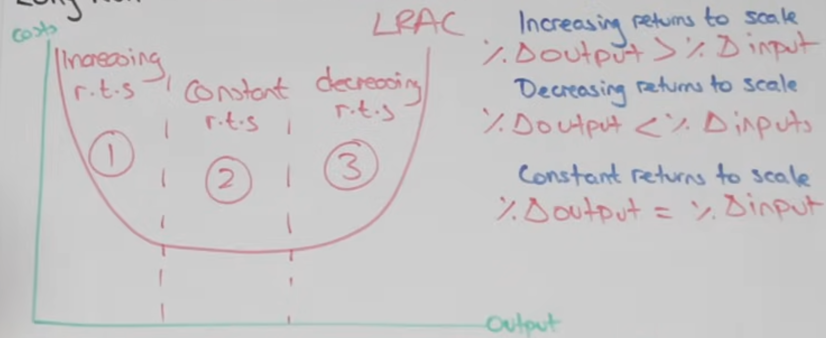
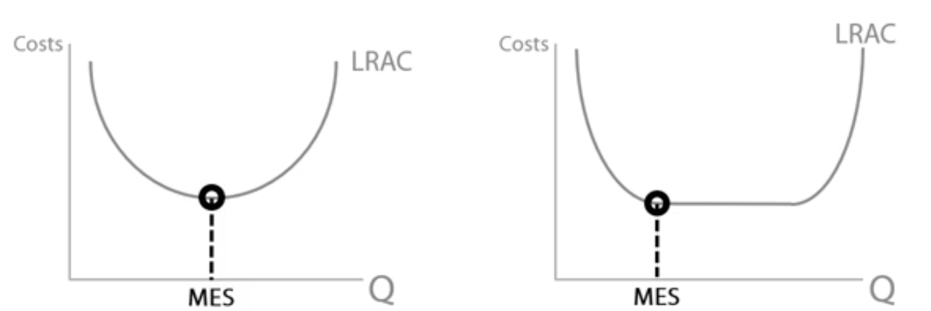
Long run average cost (LRAC) curve

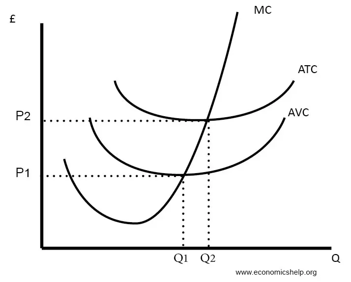
Costs + revenues diagram

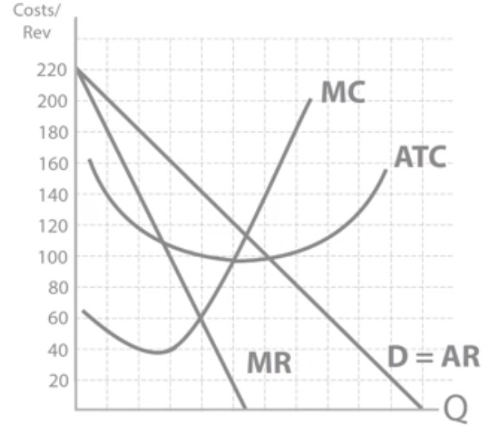
Minimum efficient scale (MES)

The lowest level of output required to fully exploit economies of scale.

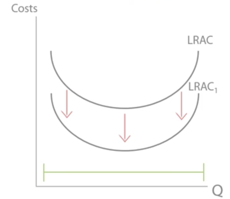
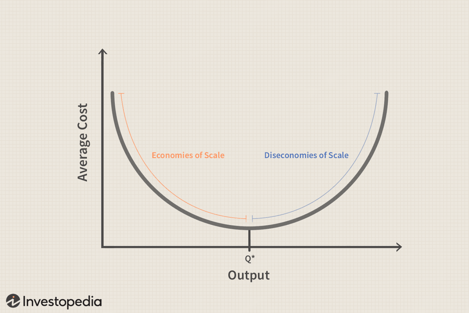
Economies of scale

Internal economies of scale

AC = TC↑/ Q↑↑↑

A reduction in LRAC as output increases.

Within a businesses control to reduce LRAC as their output increases.

TYPES:

Risk-bearing

Managerial

Financial

Purchasing

Technical

Marketing

Richard’s Mum Flies Past The Moon

Risk-bearing economies

Firm gets larger→spread opportunity cost (risk) over larger range of output→ cost per unit of output decreases.

Managerial economies

Firm gets larger→employ specialist managers with specialist skills→boost productivity of workers→increases quantity + therefore output

Financial economies

Firm gets larger→negotiate lower rates of interest from bank as they are profitable + have proven success (lower risk)→ reducing costs

Purchasing economies

Firm gets larger→able to buy raw materials in bulk by negotiating unit discounts→lower AC per unit

Technical economies

Firm gets larger→invest in specialist machinery→boost efficiency + productivity→more output

Marketing economies

Bigger firms→bulk buy advertisements e.g. billboards by negotiating lower unit costs→spread advertising costs over larger output→reduces AC per unit

External economies of scale

As entire industry grows, average cost for business decreases due to larger factors occurring outside the business.

Better transport infrastructure: e.g. new roads, airports, →reduces TC for firm as it’s cheaper to transport + access raw materials→reduces AC

Component suppliers move closer: large firm→in their interest to move closer to firm→reduce transport costs + TC

Diseconomies of scale

AC = TC↑↑↑/ Q↑

An increase in LRAC as output increases.

3 C’s and an M

Control: Firm grows→ harder to control workforce→workers slack off→productivity decreases

Communication: Firms grows→harder+slower to communicate + send messages between CEO’S + workers→reduce productivity

Coordination: Firm grows→difficult for different departments to coordinate + working in same way→decreases productivity

Motivation: Firm grows→workers feel like they’re not value→demotivated to work→productivity decreases.

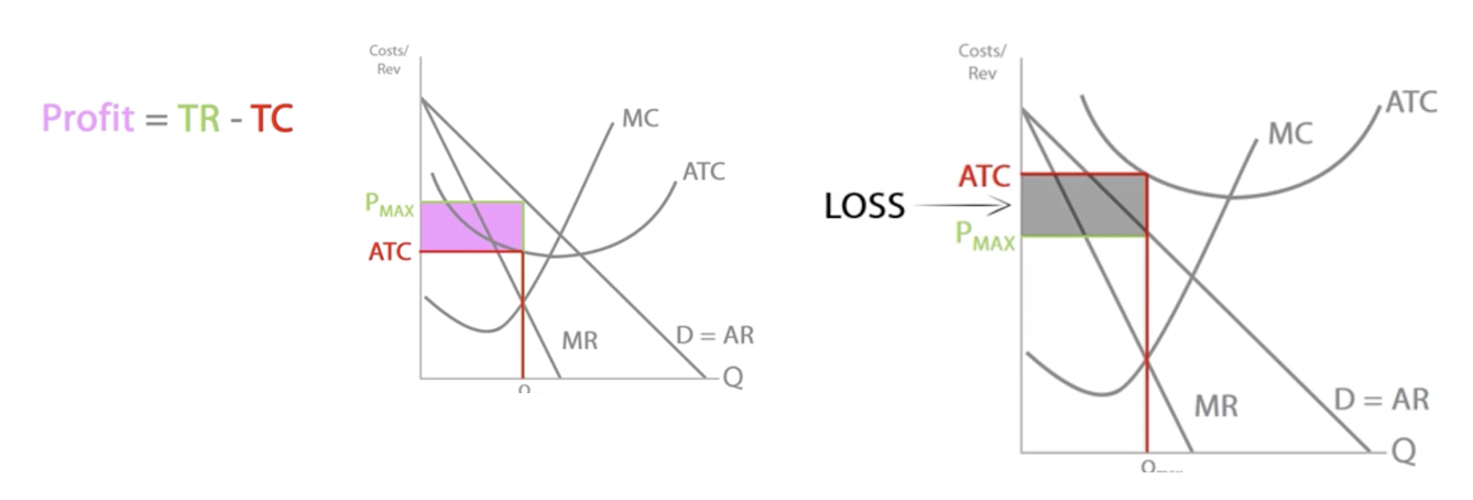
Profit

Economic profit = TR - TC

TC: Physical costs (TFC, TVC) + Opportunity costs

Normal profit, supernormal profit, subnormal profit

Normal profit: The minimum level of profit required to keep FoP in their current use + cover TC. Economic profit = 0

AR = AC

Supernormal profit: Any profit made above normal profit.

AR>AC

Economic loss: Any profit made below normal profit. Profit made is not enough to cover the opportunity cost of production.

AR<AC

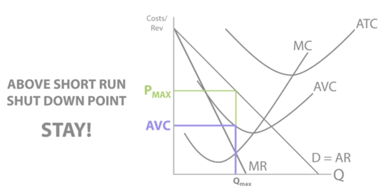
Short run shut down point

Price(AR) = AVC

If price(AR) > AVC, firms will stay in the market(not shut down), as any revenue generated above the firms AVC can be used to pay off fixed costs.

Still gaining money on each unit sold

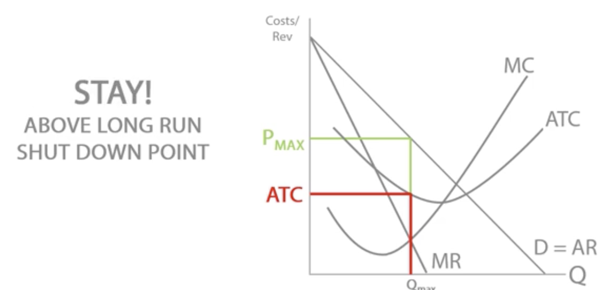
Long run shut down point

Price(AR) = ATC

as there are no fixed costs in the long run as all factors of production are variable.

If price(AR) > ATC, firm will stay in market as it’s still making profit on each unit sold.