AP STAT UNIT 1-6

association

- now two set of data compare and relate to each other

-Trends in the data

Dot plots

- one dimensional

- put a dot every time a value is obtained

4 things you should always describe

-shape

-center

-spread

-outliers

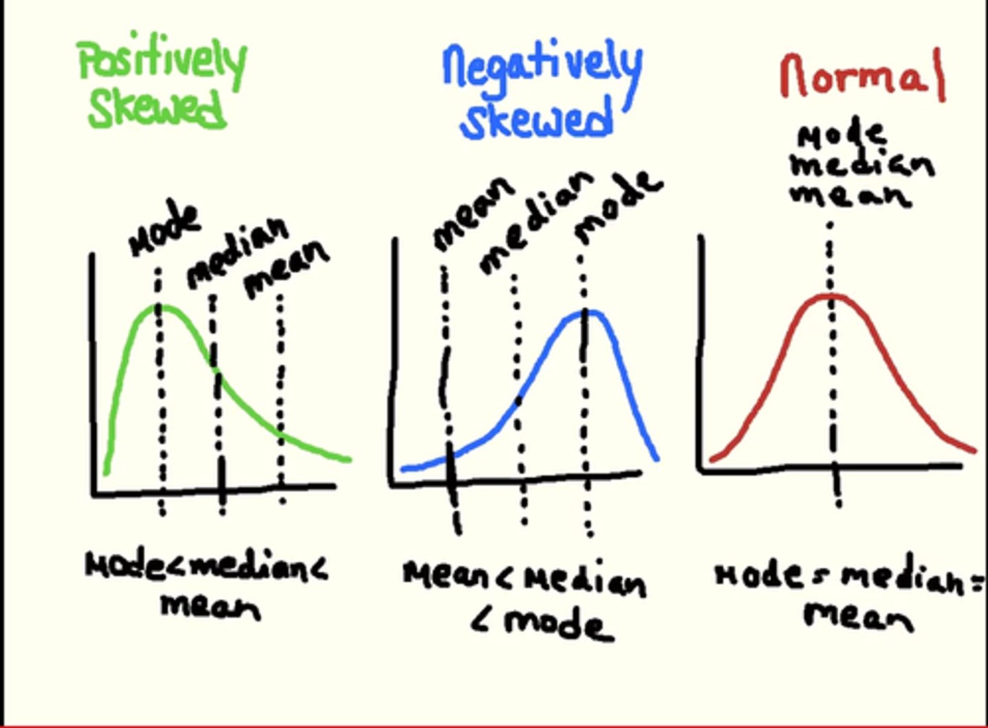
Words for shape

-Shew: data more compact on one side

- unimodal vs multimodal

Histogram

- Show distrubution of quantitative data in graph similar to a bar graph

Median

When there are outliers use to get center

Mean

Always get toward shew

Standard deviation

How spread out from the mean the data is

Organizing a stats problem

-state: what are you trying to find sample population st.dev

-plan: how do I get to that answer

-do: do the plan

-conclude: draw conclusion and properly label answer

Percentile

Percent that data piece is better than or equal to

Z score

The # of st.dev away from the mean a piece of data is

Z=

X-mean/st.dev

When mult/div a constant

-center, spread, 5 # summary also change by constant

-st.dev change by constant

-shape stays same, but spread still changes

When adding/subtr a constant

-center, spread, 5 # summary shift by the constant

- St.dev, stay same

-Shape stay same

Density curve

-Is always on or above horizontal axes

-has area exactly 1 underneath it

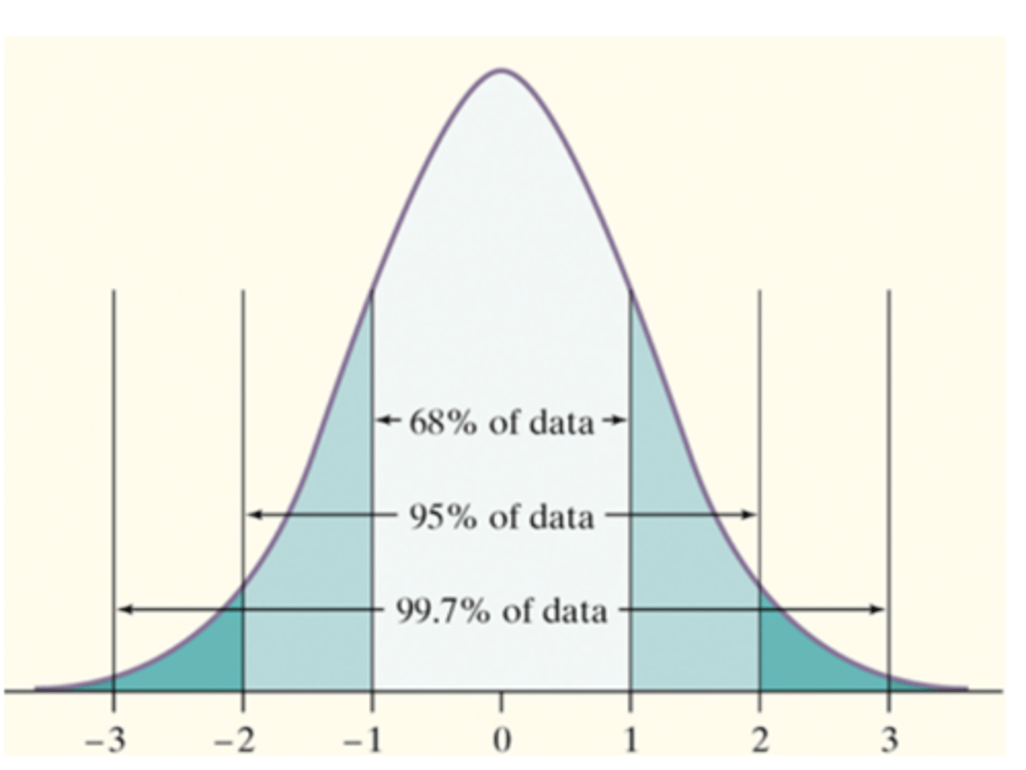
Normal curves

-symmetric, unimodal, bell shaped

-can be completely described by mean and standard dev.

Normal

-unimodal

-symmetrical

-68,95,99.7 rule

Normal probability plot

Convert all data into expected Z score and plot it

Explanatory variable

May help explain or predicted the outcome/response variable, x/input/independent variable

Response variable

-the outcome of the study

-y/output/independent variable

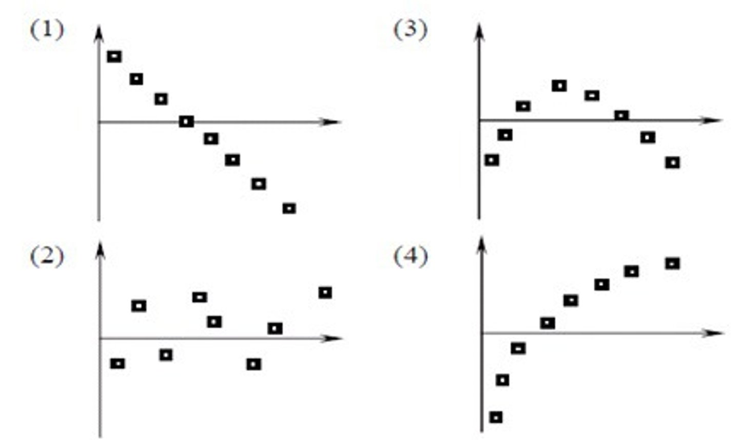
Describe scatterplots

1)direction- positive/negative/no association

2)Form- straight/ curves; clustered/uniformed

3) strength- how close data is to the form

4) Outliers

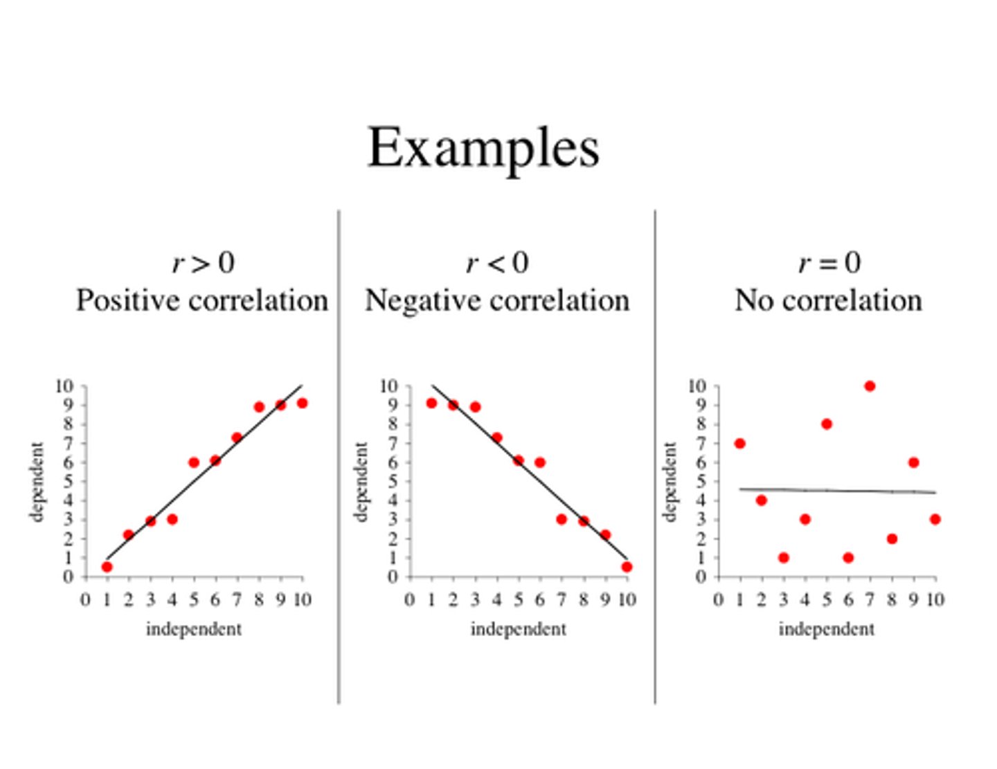
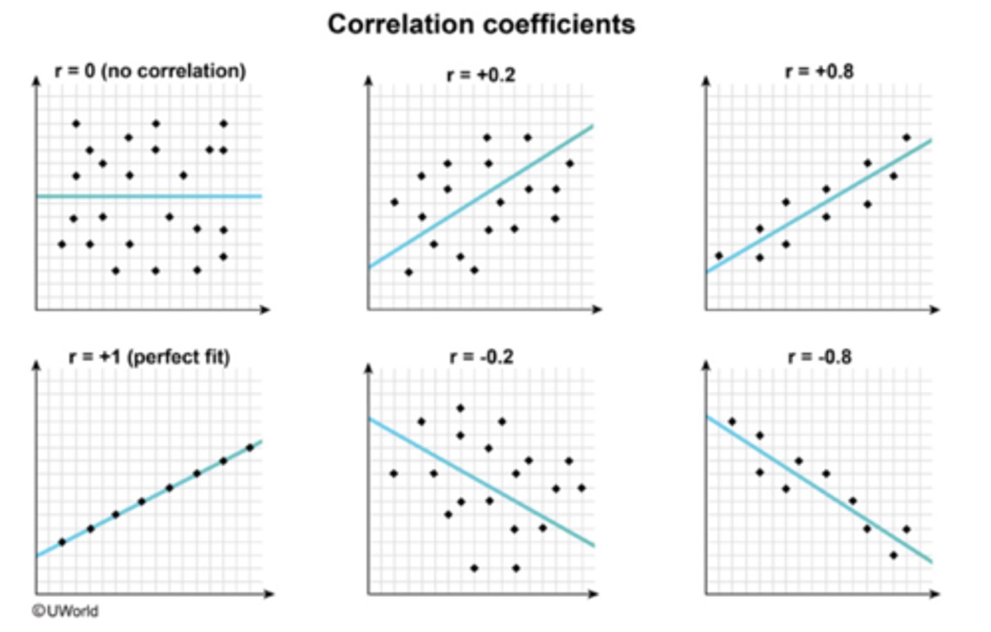
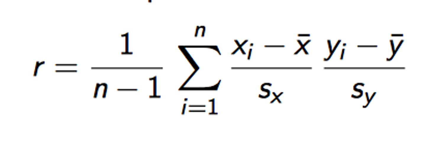
r-value

-give strength and direction

-between -1 and 1

-neg r value= neg association

-pos r value= pos association

- the close +/-1, the stronger

Formula for r-value

residual

-The difference between an observed and predicted value

y hat

predicted value

interpopulation

within data range/ more accurate

extrapolation

outside data range/ less accurate

residual plot

-scatter plot of all residual

-help us see if data is linear or not

- can them tell if linear model is linear or not

-more random, the better a linear model is

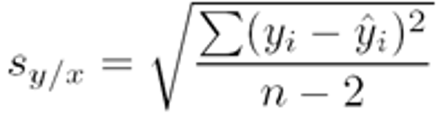
s=

-st.dev of the residuals

-Gives the typical error of a prediction using that linear regression model

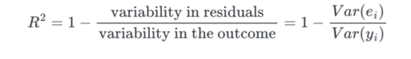
r^2

tells you the % of variance that is accounted for by the linear model

tips and tricks

1) it is important to know which is explanatory variable and response variable

2) correlation and linear regression lines only describe linear relationship/ always plot data to seeother association

3) correlation and least squared regression are not very resistant

Probability

a proportion/decimal between 0 & 1

Law of large numbers

the more you test something, the more likely your result are around its probability

simulation

-running an accurate test based on the probability of a situation

-do not tell us if things were actually done fairly or set up equally, they tell us how likely certain result appear if they were

Sample space

a list of all possible outcomes

probability model

description of the sample space S and probability of each outcome

event

- a collection of outcomes from a chance process

-a subset of the sample

-given titles of capital letters like A,B,C,D....

Probability of one

P(A)+(PnotA)

Basic rules of probability

-The prob of an event is always between 0 & 1

-All possible outcomes added together must be = 1

- If all outcomes are equally likely, the prob of an events is found

-probability of an event not happening is equal to 1-probthat it does

-If two events have no outcomes in common, the probability once occurs is the sum of their probabilities

+called mutually exclusive or disjoint

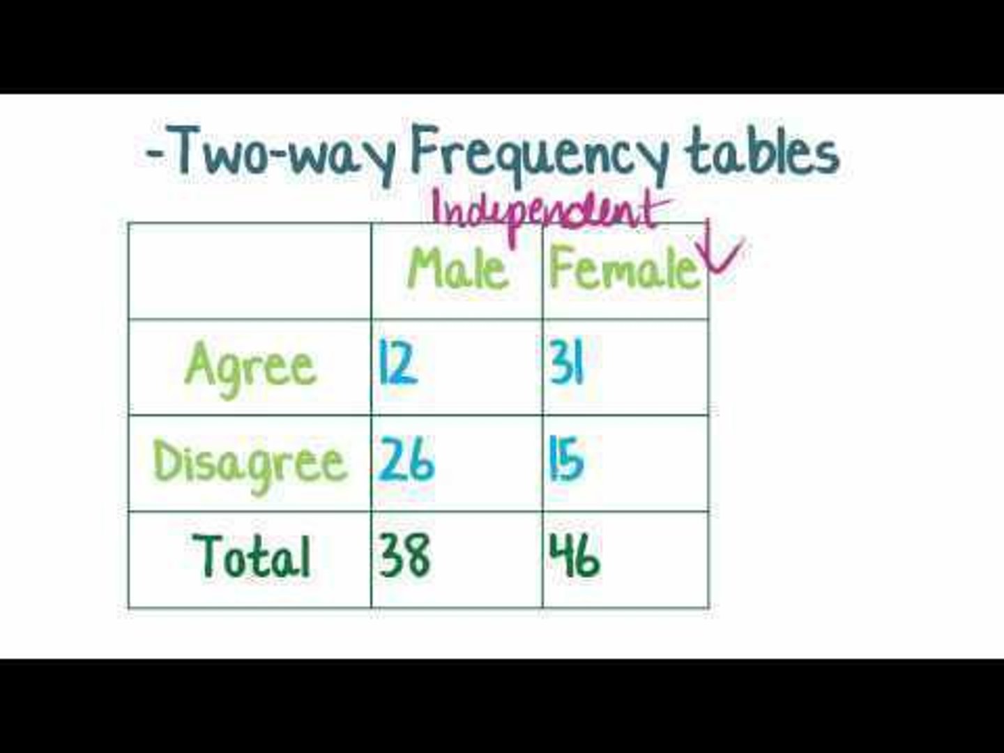
Two way tables

p(AorB)= P(A) + P(B) - P(A & B)

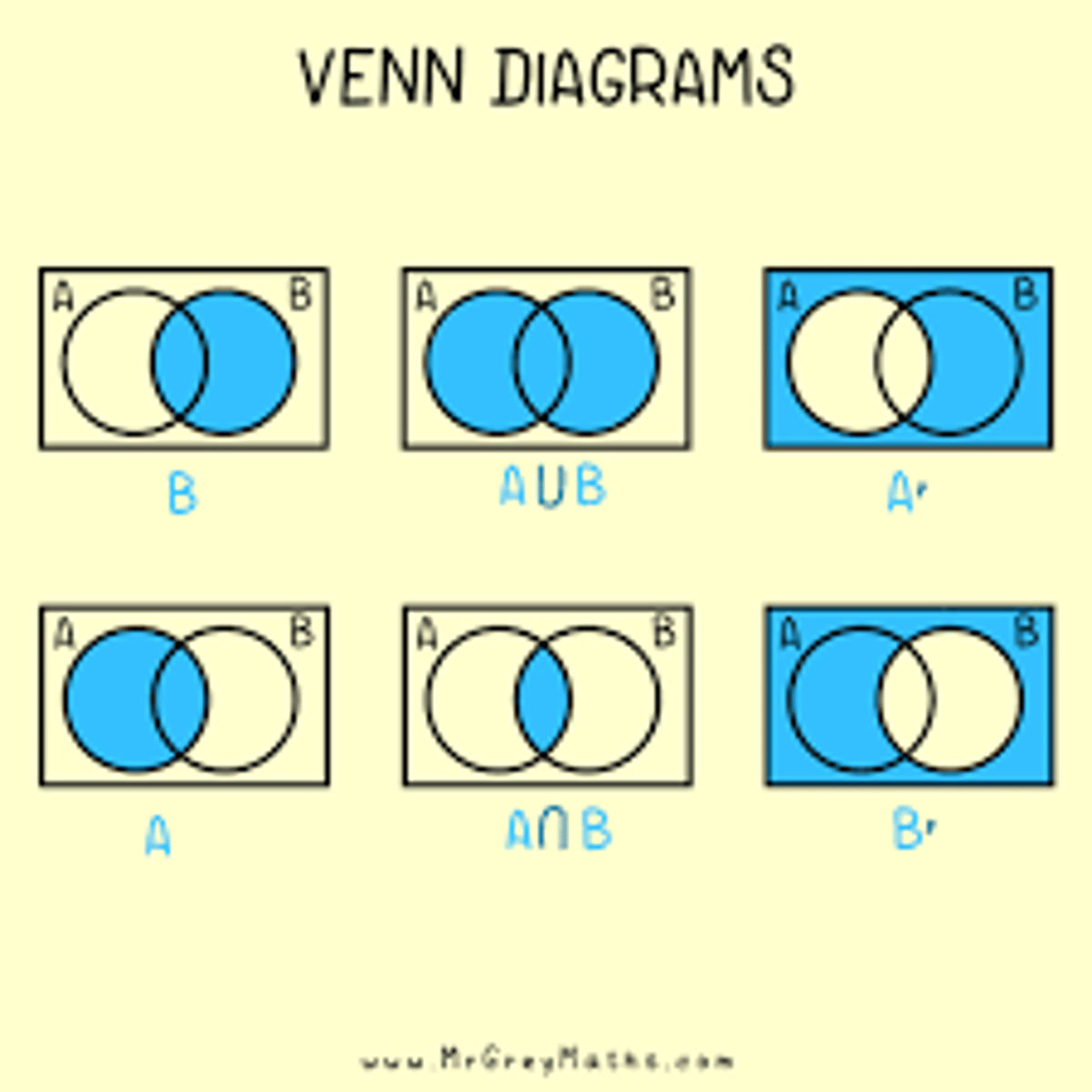
Venn Diagram

A n B

A u B

Conditional prob

P(A|B) = P(A and B) / P(B)

-The probability that one event happens given another one already did

-prob of A given B

Independent events

-Two events are independent if one event does not change the probability of the other happening

-If two events are mutually exclusive they CANNOT be independent

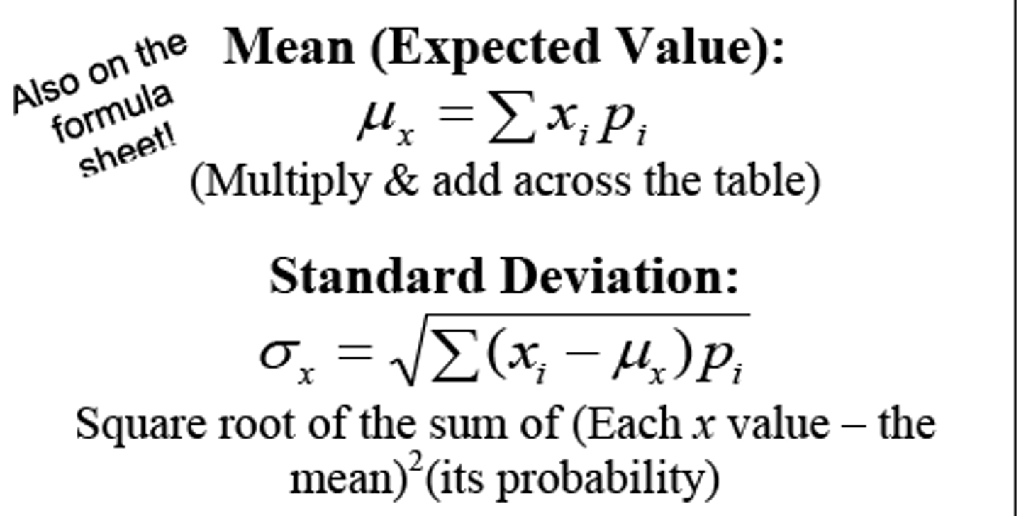
Random variables

-a numerical value that describe the outcome of some chance process

-probability distribution show the chances of random

Discrete random variable

-a fixed set of possible values with gaps in between them

-must have probabilities between 0 & 1 and add up to 1

Variance of discrete variables

-amount a value is different from the expected

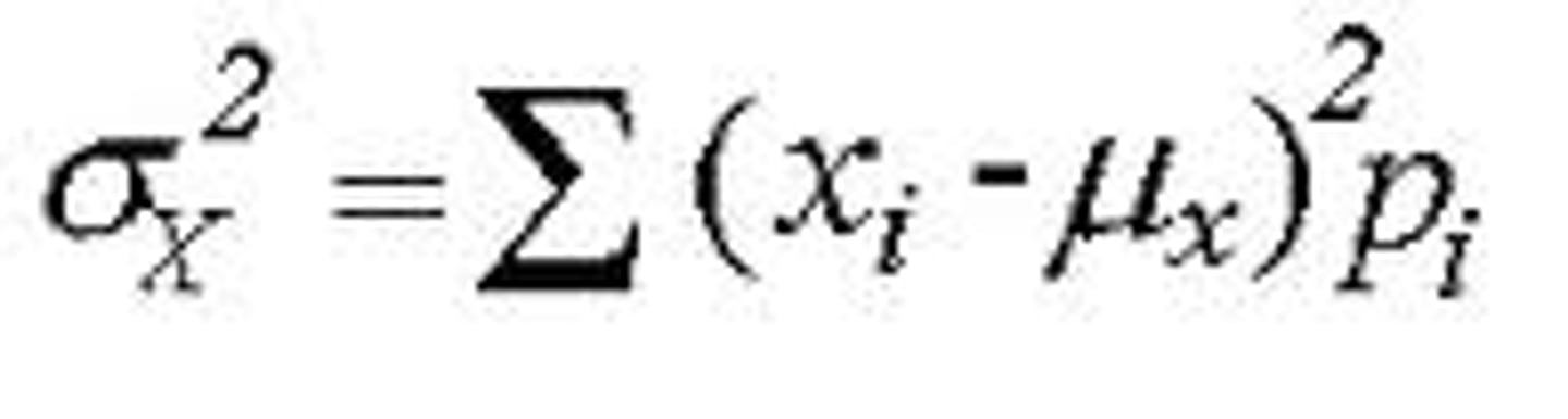
Standard deviation

the square root of the variance

Continuous randoms variable

-any # of outcomes

Multiplying a random variable by a constant

-multiplies center and location (mean, median, quartiles, etc) by same #

-Multiply spread (range, IQR, st.devi,etc)

-Does not change shape

-Variance is changed by the (constant)^2

add/subtract

-measures of center and location (mean, median, quartiles, etc) move by what we add/subtr

-Shape and spread (range, IQR, st.dev) don't change

If we add a and multiply by b

-new data would be y=a+bc

-Shape stays same as long as b>0

-Mean= a+bmean

Independent Random Variables

-knowing one has no influence on the other

-allows separate events to be multiplied

range

rangex+rangey

All these work the same when subtracting random variables

Binomial setting

-two outcomes: success and failure

-Independent: knowing one result doesn't influence others

-Number: the number of trials n is set in advance

-Success: the p of success remains constant

Binomial random variable

count of success and expected successes in a binomial setting

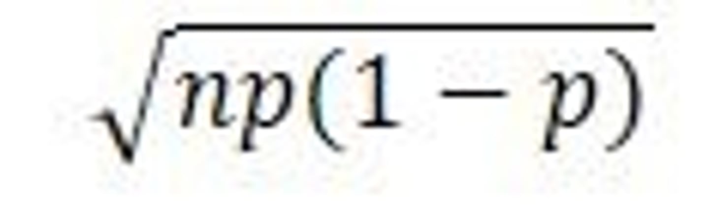
Binomial distribution

parameters n & p for a binomial setting and how possible X outcomes range from 0 to n

binomial coefficient

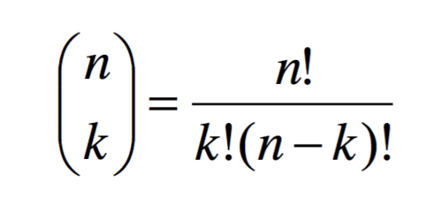
number when binomial

mean= np

10% condition

if you do on SRS of a population using less than 10% of the population, you can do binomial distribution

Large count condition

X will be approximately normal if np>/= 10

Geometric settings

-perform independent trials w/some chance of success until we get a success

-Geometric variable y is the # of trials somethings takes

geometpdf(p,k)

p(y=k)

geometcdf(p,k)

p(y

binomialpdf (n,p,k)

p(x=k)

binomialcdf (n,p,k)

p(x<=k)