MOC: turing machines

Turing Machine, informally

The definition of a Turing machine in this course consists of a two-way-infinite tape which starts at the left of the input string.

• The machine starts in state s with the tape head pointing to the first symbol of the finite input string. (Everything to the left and right of the input string is initially blank.)

• The machine computes in steps, each depending on the current state (q) and symbol being scanned by tape head (0)

• An action at each step is to: overwrite the current tape cell with a symbol; move left or right one cell; and change state.

Turing Machine, formally

A Turing machine is specified by a quadruple M = (Q, Σ, s, δ) where

• Q is a finite set of machine states;

• Σ is a finite set of tape symbols, containing distinguished symbol _, called blank;

• an initial state s ∈ Q;

• a partial transition function δ ∈ (Q × Σ)⇀(Q × Σ × {L, R})

The machine has finite internal memory. It can remember which state it is in, nothing more. At each step of the computation, the machine reads the symbol currently under the tape head. If the machine is currently in state q and reading symbol a then δ(q, a) tells the machine what to do next. If δ(q, a) is undefined, the machine simply halts. Otherwise, δ(q, a) = (q′ , a′ , d) for some state q′ , symbol a′ and direction d. The machine overwrites the current cell with the symbol a ′, moves along the tape in direction d (L for left, R for right), and changes its state to q′.

definition: Turing Machine configuration

A Turing Machine configuration (q, w, u) consists of

• the current state q ∈ Q;

• a finite, possibly-empty string w ∈ Σ∗ of tape symbols to the left of tape head;

• a finite, possibly empty string u ∈ Σ∗ of tape symbols under and to the right of tape head. Є denotes the empty string.

The configuration only describes the contents of tape cells that are part of the input or have been visited by the Turing machine. Everything else is blank.

definition: initial configuration

An initial configuration is (s, Є, u), for initial state s and string of tape symbols u.

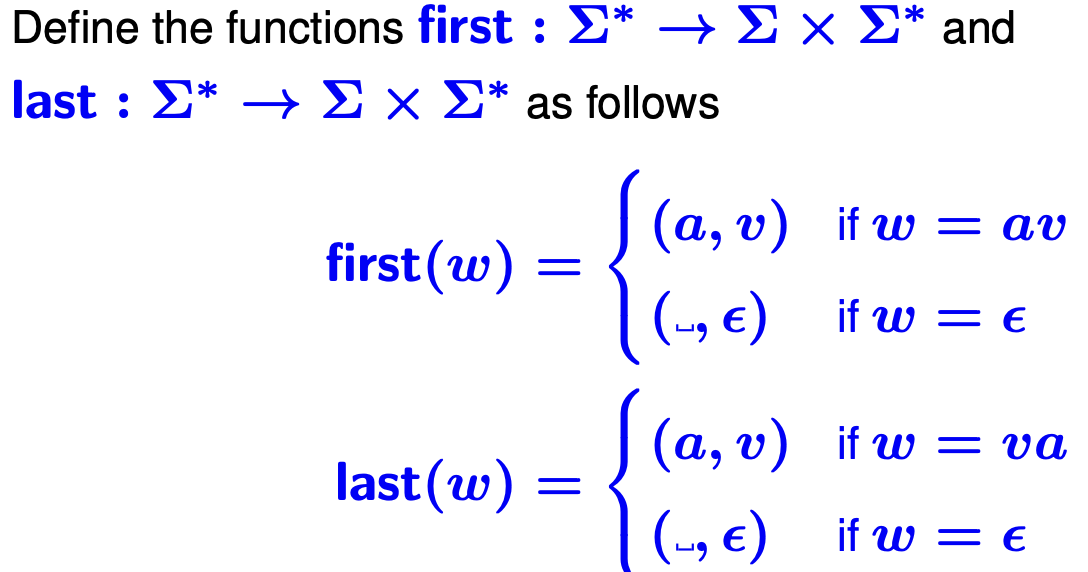
definition: first and last functions

These functions split off the first and last symbols of a string, splitting off if the string is empty.

definition: Turing Machine computation

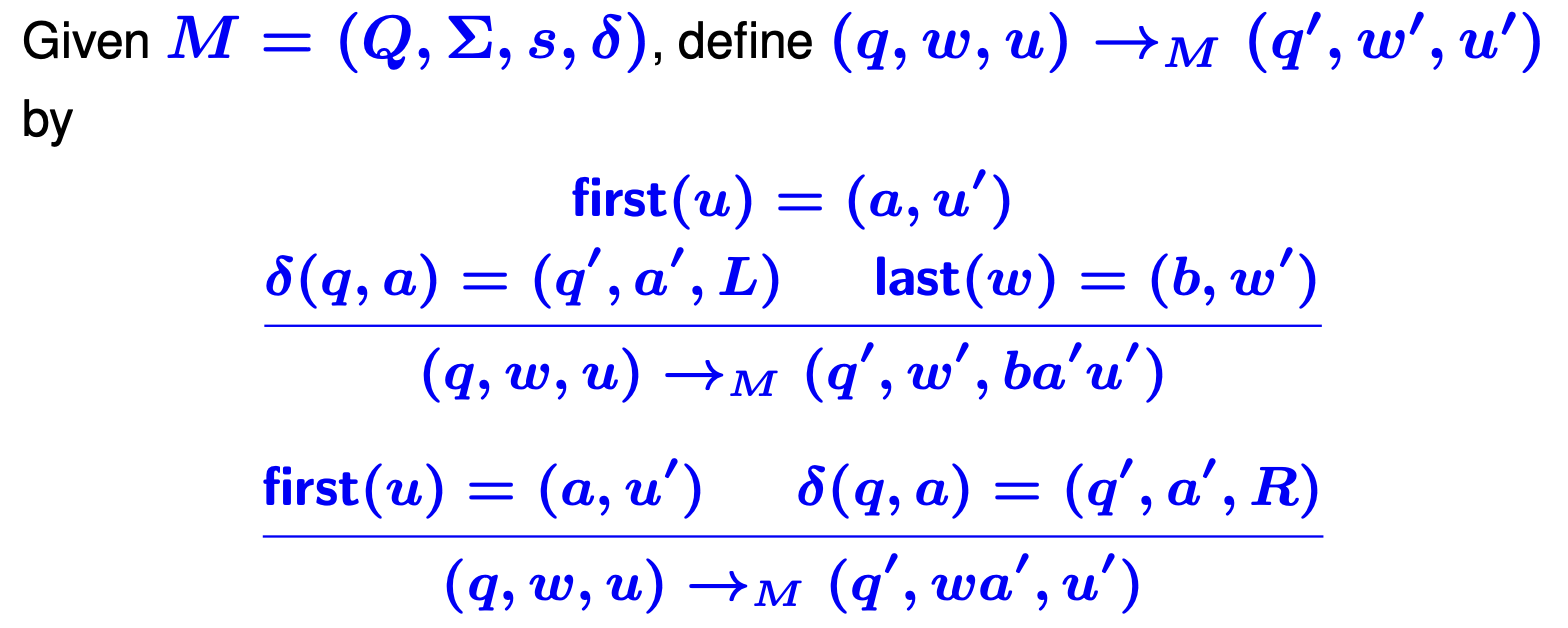
definition: configuration normal form

We say that a configuration (q, w, u) is a normal form if it has no computation step. This is the case exactly when δ(q, a) is undefined for first(u) = (a, u′).

definition: Turing Machine computation

A computation of a TM M is a (finite or infinite) sequence of configurations c0, c1, c2, . . . where

• c0 = (s, Є, u) is an initial configuration

• ci →M ci+1 holds for each i = 0, 1, . . ..

The computation

• does not halt if the sequence is infinite

• halts if the sequence is finite and its last element (q, w, u) is a normal form.

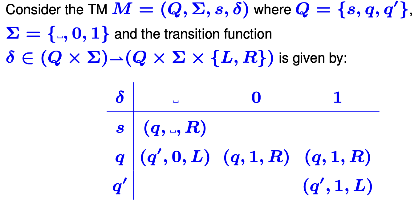
example: Turing Machine

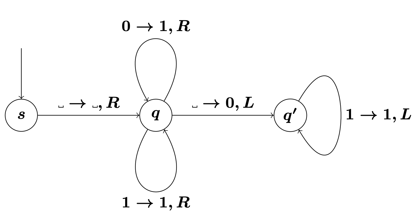
graphical representation of Turing Machines

Construct a graph representing a TM:

• Nodes: states q ∈ Q,

• Edges: representing the transition function: For ((q, a), (q ′ , a′ , D)) ∈ δ with q, q′ ∈ Q, a, a′ ∈ Σ and D ∈ {L, R} there is a link from q to q ′ labelled by a → a ′ , D, and

• Initial state: s ∈ Q indicated e.g. by an (unlabelled) edge.

example: graphical representation of Turing Machine

theorem relating TMs and RMs

Theorem: The computation of a Turing machine M can be implemented by a register machine

Proof (sketch).

Step 1: fix a numerical encoding of M’s states, tape symbols, tape contents and configurations.

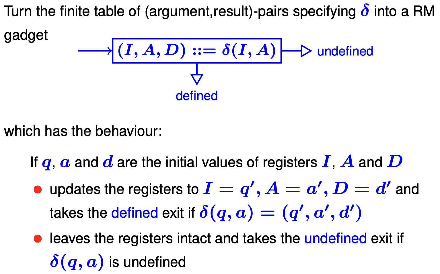
Step 2: implement M’s transition function (finite table) using RM instructions on codes.

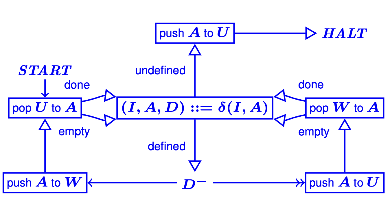
Step 3: implement a RM program to repeatedly carry out →M.

Step 1: fix a numerical encoding of M’s states, tape symbols, tape contents and configurations.

• Identify states and tape symbols with numbers: Q = {0, 1, . . . , n} Σ = {0, 1, . . . , m} where s = 0 and _ = 0

• Code configurations c = (q, w, u) with three numbers:

• q, the state number

• ceil([ai, . . . , a1]) where w = a1 · · · ai

• ceil([b1, . . . , bj ]) where u = b1 · · · bj.

[The reversal of w makes it easier to use our RM programs for list manipulation.]

• Identify directions with numbers: L = 0, R = 1

Step 2: implement M’s transition function (finite table) using RM instructions on codes

Step 3: implement a RM program to repeatedly carry out →M

converse of TM-RM theorem

The converse holds: the computation of a register machine can be implemented by a Turing machine.

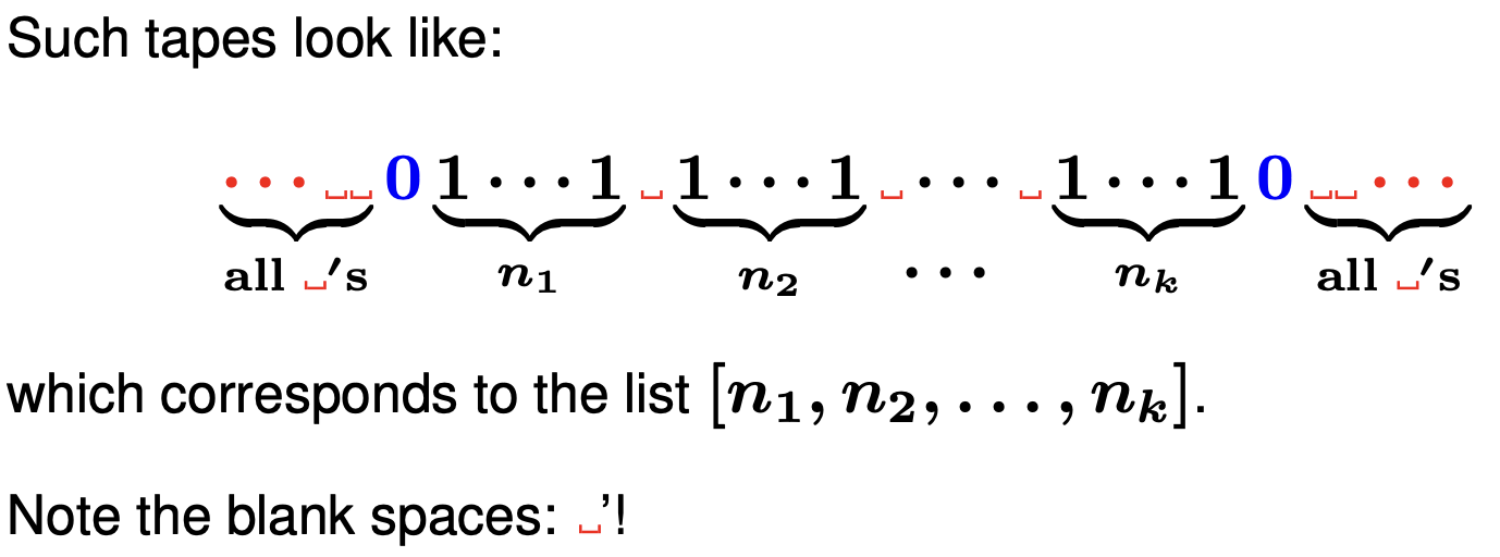
definition: tape encoding lists of numbers

A tape over Σ = {_, 0, 1} codes a list of numbers if precisely two cells contain 0 and the only cells containing 1 occur between these

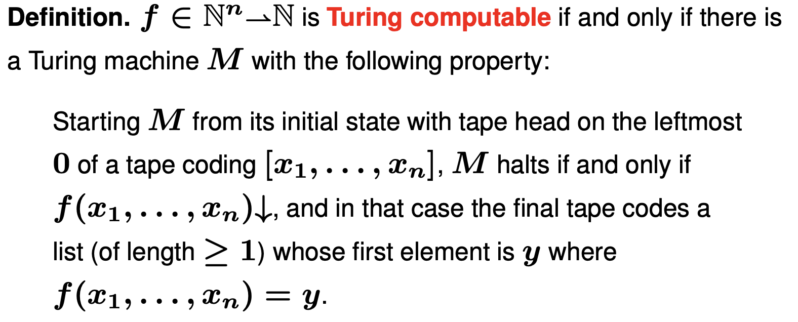
definition: Turing computable function

theorem: Turing computable functions

Theorem: A partial function is Turing computable if and only if it is register machine computable.

Proof (sketch): We’ve seen how to implement any TM by a RM.

Hence f TM computable implies f RM computable.

converse theorem: Turing computable functions

For the converse, one has to implement the computation of a RM in terms of a TM operating on a tape coding RM configurations. To do this, one has to show how to carry out the action of each type of RM instruction on the tape. It should be reasonably clear that this is possible in principle, even if the details are omitted (because they are tedious).

Church-Turing thesis

Every algorithm [in intuitive sense] can be realized as a Turing machine.

I.e. anything that is algorithmically computable is computable by a Turing machine