AP Stats Final Review (Ch. 1-6)

Goal for final: 73.57%

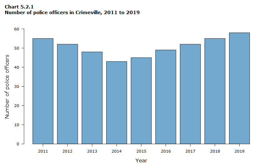
Bar graph

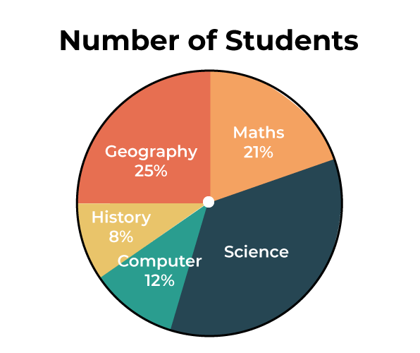
Pie chart

3 ways that a graph can be misleading

1. violating the area principle

2. the vertical axis doesn’t start with zero

3. uses pictures

Categorical variables are displayed…

in a bar graph or pie chart

Quantitative variables are displayed…

in a dotplot, stemplot, or histogram

Stemplot

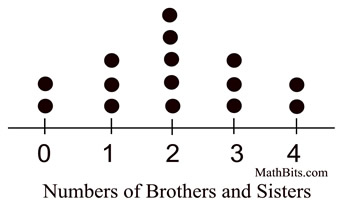
dotplot

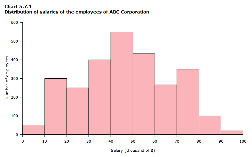
histogram

First S in SOCS

Shape

O in SOCS

Outlier

C in SOCS

Center

Second S in SOCS

Spread

If we are finding the CENTER in a APPROXIMATELY SYMMETRICAL distribution…

we use the mean

If we are finding the CENTER in a SKEWED distribution…

we use the median

If we are finding the SPREAD in a APPROXIMATELY SYMMETRICAL distribution…

we use the standard deviation

If we are finding the SPREAD in a SKEWED distribution…

we use the IQR

Identifying outliers in a distribution

1.5IQR

Lower bound for outliers

Q₁ - 1.5IQR

Upper bound for outliers

Q₃ + 1.5IQR

boxplot

Variance equals…

st. dev.²

Standard deviation equals…

√variance

Interpreting the standard deviation

The (context) typically varies (s_x) from the mean of x

z-score formula

(x - mean) ÷ st. dev.

Interpreting the z-score

(Context) is (z-score) standard deviations (above/below) the mean (context)

Adding/subtracting a constant…

affects the center

Multiplying/dividing by a constant…

affects center AND spread

Empirical rule

68-95-99.7

Normal distribution on a calculator

normalcdf(lower, upper, µ, σ)

Z-score on a calculator

invNorm(area to the left, µ, σ)

Scatterplot

D in DOFS

Direction (positive/negative)

O in DOFS

Outlier

F in DOFS

Form (linear/curved/none)

S in DOFS

Strength (strong/moderate/weak)

When describing a scatterplot…

you MUST interpret the Direction

Interpreting the correlation

There is a (weak/moderate/strong), (positive/negative) linear relationship between x and y. (DOFS without O)

LSRL formula

y^ = a + bx (prediction)

Interpreting the slope of LSRL

For every 1 (unit) increase in x, our model predicts an (increase/decrease) of (b units) in the y

Interpreting the y-intercept of LSRL

If x is 0 (units), our model predicts a y value of (a units)

residual formula

Actual - Predicted

Interpreting the residual

The actual y is (amount) (higher/lower) than predicted based on x

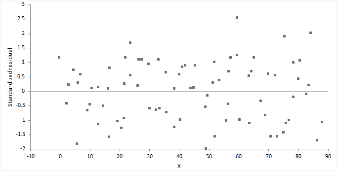
Residual plot

A linear model is appropriate…

if the residual plot shows random scatter

Interpreting the standard deviation of residual (s)

If we use this model to predict y from x, our predictions will typically be off by about (s units of y)

Interpreting the coefficient of determination (r²)

(r²)% of the variation in y is due to x

convenience sample

choosing individuals from the population who are easy to reach

voluntary sample

people decide whether to join the sample in response to an open invitation

undercoverage

occurs BEFORE the sample is chosen

nonresponse

occurs AFTER the sample is chose

response bias

a pattern of incorrect responses

wording of questions

questions that can influence someone’s answer

Choosing SRS with Technology (simple random sample)

1. Label (context)

2. randIntNoRep(lower, upper, n)

Choosing SRS with Table D (simple random sample)

1. Label (context)

2. Moving horizontally from left to right picking n digit numbers, skip numbers outside range and repeats until you get x numbers.

stratified random sample

splitting the population into sub-groups (strata)

Describing stratified random sample

1. Label x₁ 1-n, …

2. x₁: randIntNoRep(lower, upper, n)

x₂: randIntNoRep(lower, upper, n)

cluster sample

classifying the population into groups of individuals that are located near each other

Describing cluster sample

1. Label (context)

2. randIntNoRep(lower, upper, n)

systematic random sample

randomly selecting one of the first k individuals and choosing every kth individual

k in systematic random sample

population ÷ sample

Describing systematic random sample

1. Label (context) in x_{1, …}

2. k = population ÷ sample

3. randInt(lower, upper(k), n) to pick first individual , then every kth individual thereafter

observational study

observing the individuals and measuring responses

experiment

imposing treatment on individuals and measuring responses

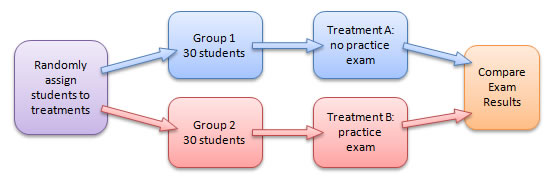
Completely randomized design

Inference about population

individuals were randomly selected

Inference about cause and effect

individuals randomly assigned to groups

Interpreting probability as a long run frequency

If many, many (context) are randomly chosen, about x% of them (context)

Performing a simulation

State, Plan, Do, Conclude

State

What is the probability that…

Plan

Label (context). Find # different n digit numbers from (line) moving horizontally from left to right in Table D and record (context). Skip numbers that repeat within a simulation or are outside the range).

Do

I will perform many repetitions of this simulation

Conclude

In our simulation, about n% (context). There is convincing evidence that…

Mutually exclusive

P(A and B) = 0

Complement rule

P(A^c) = 1 - P(A)

Addition rule for mutually exclusive

P(A or B) = P(A) + P(B)

Conditional probability formula

P(A l B) = P(A and B) / P(B)

General multiplication rule

P(A and B) = P(A) x P(B l A)

Use tree diagram

1. given conditional probabilities

2. given sequences of events

3. given lots of percents

Use two-way table

1. given counts of people

Multiplication rule for independent events

P(A and B) = P(A) x P(B)

The 2 requirements for probability in Ch. 6

1. Every probability is a number between 0 and 1

2. The sum of the probabilities is 1

The meaning of P(X ≥/≤ n)

Probability that (context) is at least/most n

Mean (expected value) of a Discrete Random Variable Formula

µ(x) = E(x) = x_ip_i+…

Standard deviation of a Discrete Random Variable Formula

σ(x) = √(x_i - µ_x)² p_i

Multiplying/dividing by constant

affects the mean and st. dev. of the distribution

Adding/subtracting a constant

affects the mean of the distribution