AP Stats Unit 2 Quiz

CDOFS =

• Context (explanatory and response variable with units)

• Direction (positive/negative)

• Obvious?

  • Influential points

    • Outliers

    • High leverage points

  • Etc.

• Form (linear or nonlinear)

• Strength |r| (weak < 0.5 < moderate < 0.7 < strong)

Interpret the coefficient “r”

r =___. There is a (strong/moderate/weak) (positive/negative) relationship between explanatory variable and response variable. (Note: you cannot determine form from a correlation coefficient only)

Interpret the coefficient of determination “r²”

• ___% of the variation in the response variable can be explained by the linear relationship with explanatory variable. 

• ____% of the error in is accounted for

Interpret the slope “b”

• For each additional/(increase by 1 ____ in) explanatory variable, the predicted response variable will (increase/decrease) by ___. 

Interpret the y-intercept “a”

The predicted response variable when explanatory variable = 0 is ___. 

• also interpret if this value makes sense in the context

Interpret residual

The residual is ___. This means that the actual response variable is ___

• (less than/more than) predicted based on explanatory value of observation. 

• (less than/more than) the predicted explanatory value of observation. 

Interpret standard deviation of the residuals “s”

s = ___. When using the least-squares regression line with x = explanatory variable to predict y = response variable, ***our predictions will typically be off from the actual data by ___.

Interpret residual plot

A linear model (or whatever the current model is) (is/is not) appropriate because there is (not an obvious/an obvious) pattern in the residual plot. 

explanatory(independent) variable

the variable that predicts, explains, or influences a trend in the response variable. This is the x - value

response (dependent) variable:

The measured outcome. Responds to trends in the explanatory variable. This is the y-variable

positive correlation

as the x-values increase, the y-values also tend to increase

negative correlations

as the x-values increase, the y-values tend to decrease

least squares regression line (LSRL):

• straight line that roughly puts half of your data above it and half below it

• makes the sum of the squared residuals as small as possible

strong correlation interpretation:

• data is close to the LSRL

• the LSRL is a good model for the data

• if you used the LSRL to predict new data, you would make close predictions

weak correlations interpretation:

• data is far from the LSRL

• the LSRL is a “meh” model for the data

• if you used the LSRL to predict new data, you may be quite a bit off

correlation coefficient (r):

A number between -1 and 1 that tells you the strength and direction of correlation

(-1 < r < 1)

• the closer to -1 or 1, the stronger the relationship

• the closer to zero, the weaker the relationship

• -1 and 1 only occur in case of perfect linear relationship

• **only used to describe linear relationship

properties of the correlation coefficient ( r ):

1. requires that both variables be quantitative

2. makes no distinction between explanatory and response variables

3. does not change when we change the units of measurement of x, y or both

4. has NO UNIT of measurement

residuals

distance between each data point of response variable and predicted value in the linear regression (y-distance between the point and the line)

The “error” between the prediction and actual

• residual = actual - predicted = y - ŷ

equation for LSRL and variable meanings

ŷ = a + bx

• a = y intercept

• b = slope

• ALWAYS LABLE VARIABLES

equation for “a”

ȳ - b(x̄)

y mean - slope ( x mean)

equation for “b”

r * (Sy)/(Sx)

correlation coefficient * (standard deviation y)/(standard deviation x)

pos. residual value =

actual value is higher than model’s prediction

neg. residual value =

actual value is lower than model’s prediction

what should the residual plot look like for a good fit model?

• be centered at zero

• have no pattern

• look random

• only random scatter

properties of LSRL

• always goes through (x mean, y mean)

• is a “see-saw” centered at (x mean, y mean)

low-leverage points:

• close to x mean

• less pull on see-saw; don’t effect LSRL much

high-leverage points:

• far from x mean

• have much larger or much smaller x values than the other points

• have a high effect on an LSRL’s slope + y-intercept

influential points:

• points that if removed change the slope, y-intercept, correlation, r², or SD of residuals substantially

• outliers and high leverage points are often influential in regression calculations

outlier

is any point that does not follow the pattern of the data and has a large residual

• change correlation

high leverage influential points

• unusually high x value

• changes slope/y-int

• not outlier because low residual (close to LSRL)

low leverage influential

• central x-value

• is an outlier: high residual (far from LSRL)

• lowers r (correlation coefficient)

both outlier + high leverage influential point

• unusually high x-value

• high residual (far from LSRL)

• changes slope/y-int

• lowers r (correlation coefficient)

Where is y-int on regression table?

the top left corner number

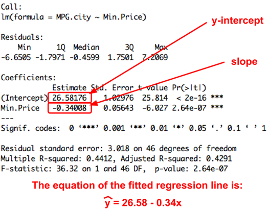
Where is slope in regression table?

the bottom left value (below y - intercept)

Where is standard deviation in regression table

It is the S value

Where is r(correlation coefficient) in regression table?

it is R-Sq value ( usually percent)

association

There is an assoication between 2 variables if knowing the value of one variable helps us predict the value of the other.

Steps for describing scatterplot:

1. Direction(pos/neg)

2. Form(linear/nonlinear)

3. Strength(weak, moderate, strong)

4. Unusual features(outliers)

   **use context

regression line

line that models how a response variable y changes as an explanatory variable x changes

extrapolation

use of a regression line for prediction outside the interval of x-values to obtain the line.

• the further we extrapolate, the less reliable the predictions become

How do you label variables or LSRL?

• put the names in the equation

• explicitly define x and y

residual plot

scatterplot that displays the residuals on the vertical axis and the values of the explanatory variable on the horizontal axis

coefficient of determination r²

measures percent reduction in the sum of squared residuals when using LSRL to make predictions rather than the mean value y

• r² measures the proportion of the variations in the response variable that is accounted for by the explanatory variable in the linear model

standard deviation of residuals “S”

measures the size of a typical residual that is, S measures the typical distance between the actual y-value and the predicted y-value

how do you undo log?

raise to power of 10

how do you undo ln

raise to power of e

How do you choose the most appropriate model?

• choose the model whose residual plot has the most random scatter

• if more than one model produces a randomly scattered plot, choose the model with the largest r²

• not advisable to us S as y values may be on different scales