Econ 1010 Chapter Ten Notes

The Firm’s Goal

A firm’s goal is to maximize profit. If the firm fails to maximize its profit, the firm is either eliminated or taken over by another firm that seeks to maximize profit.

Accounting Profit

Accountants measure a firm’s profit to ensure that the firm pays the correct amount of tax and to show the investors how their funds are being used.

Accounting Profit equals total revenue minus total cost (all types of direct costs)

Revenue = Quantity times Price

Economic Accounting

Economists measure a firm’s profit to enable them to predict the firm’s decisions, and the goal of these decisions is to maximize economic profit.

Economic profit is equal to total revenue minus total cost (measured as the opportunity cost of production)

Firm’s Opportunity Cost of Production

A firm’s opportunity cost of production is the value of the best alternative use of the resources that a firm uses in production. A firm’s opportunity cost of production is the sum of the cost of using resources:

1. Bought in the market (is an opportunity cost because there are different resources to produce some other good or service)

2. Owned by the firm (the firms OC of using the capital it owns is called implicit rental rate of capital)

3. Supplied by the firm's owner (owners supply entrepreneurship and labour and the return is normal profit (the profit entrepreneurs expect to receive). Normal profit is the cost of entrepreneurship and is an opportunity cost of production)

Implicit Rental Rate of Capital

It is made up of:

1. Economic depreciation: the change (beginning price minus new price) in the market value of a capital over a given time

2. Interest forgone: the return on the funds used to acquire the capital

Decision Time Frames

Some decisions are critical to the survival of the firm. Some decisions are irreversible.

Other decisions are easily reversed and are less critical to the survival of the firm, but still influence profit.

All decisions can be placed in two-time frames that are based on easily they can vary:

§ The short run
§ The long run

Short Run

The short run is a time frame in which the quantity of one or more resources used in production is fixed (cannot be changed). Short-run decisions are easily reversed. For most firms, the capital, called the firm’s plant, is fixed in the short run (irreversible).

Resources used by the firm (such as labor, raw materials, and energy) can be changed in the short run in order to change production.

Firms can only change production in the short run by changing variable resources

The Long Run

The long run is a time frame in which the quantities of all resources—including the plant size—can be varied.

A sunk cost is a cost incurred by the firm and cannot be changed (it cannot be recovered). Sunk costs are irrelevant to a firm’s current decisions - > examples include, new equipment, salaries, research

Increase Production in Short Run

To increase output in the short run, a firm must increase the quantity of labour employed.Three concepts describe the relationship between output and the quantity of labour employed:

1. Total product
2. Marginal product
3. Average product

Production Quantity is dependent on factors of production

Total product

Total product is the total output produced in a given period

Marginal Product

Marginal Product of labor is the change (new minus old) in total product that results from a one-unit increase in the quantity of labor employed/ hired (represents at what rate total product increases (an increasing rate or decreasing rate))

Average product

Average product of labour is equal to total product divided by the quantity of labour employed

Increase Production in Short Run Example

As the quantity of labor employed increases:

§ Total product increases
§ Marginal product increases initially but eventually decreases (10-4=6)
§ Average product decreases (10/2 = 5)

*Based on this table, it is assumed that two workers is the optimal (Law of diminishing marginal returns - > adding an additional factor of production results in a smaller increase in output)

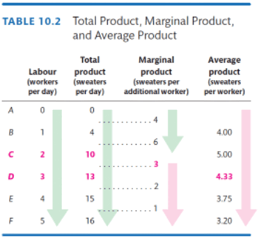
Increase Production in Short Run Example Table

#

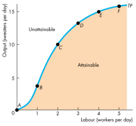
Product Curve

Product curves show how the firm’s total product, marginal product, and average product change as the firm varies the quantity of labour employed. The x axis represents the quantity of labor employed and y axis represents output.

The total product curve is similar to the PPF. It separates attainable output levels from unattainable output levels in the short run. Note: The TP curve becomes steeper at low output levels and then less steep at high output levels

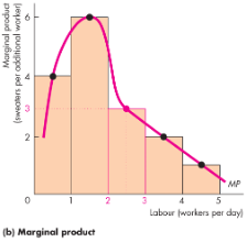
Marginal Product Curve

This curve shows the marginal product of labor and how the marginal product curve relates to the total product curve. It has an inversely U - shaped curve (initially increases, then decreases)

To make a graph of the marginal product of labor, we stack the marginal product value form very increase in one unit of labor from the product curve or in other words the height of each bar. The marginal product of labor curve passes through the mid-points of these bars.

Optimal

MP multiple Price = marginal revenue product of labour (compare this to wages).

You want MRP of Labour to equal wages (if it is more, employer will hire more workers, if it is too little, employer will fire workers)

Short-Run Technology Constraint

Almost all production processes have

§ Increasing marginal returns initially
§ Diminishing marginal returns eventually

Law of diminishing returns

As a firm uses more of a variable input with a given quantity of fixed inputs, the marginal product of the variable input eventually diminishes.

Increasing Marginal Return

Initially, the marginal product of a worker exceeds the marginal product of the previous worker. The firm experiences increasing marginal returns due to specialization and increased divisions of labor

Diminishing Marginal Returns

Eventually, the marginal product of a worker is less than the marginal product of the previous worker. The firm experiences diminishing marginal returns due to break in specialization

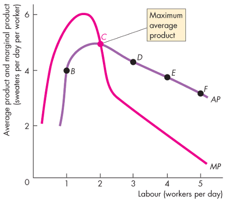
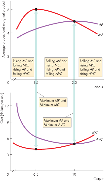
Average Product Curve

This graph shows the average product curve and its relationship with the marginal product curve.

When marginal product exceeds average product, average product increases (from 0 to 2).

When marginal product is less than average product, average product decreases (from 2 to 5).

When marginal product equals average product, average product is at its maximum (point c).


The output at which average product is a maximum is the same output at which​ average variable cost is a minimum.

Short Run Cost

To produce more output in the short run, the firm must employ more labor, which means that it must increase its costs.

Three cost concepts and three types of cost curves are
§ Total cost
§ Marginal cost
§ Average cost

*In short run there are two types of factors: fixed factors (not dependent on production or output, will never change) and variable factors (dependent on production or output, will change accordingly)

Cost depends on output/ production

Total Cost

A firm’s total cost (TC) is the cost of all resources used

Total cost equals total fixed cost plus total variable cost or TC = TFC + TVC

Total fixed cost

Total fixed cost (TFC) is the cost of the firm’s fixed inputs. Fixed costs do not change with output (not dependent on production) TFC = TC - TVC

Total variable cost

Total variable cost (TVC) is the cost of the firm’s variable inputs. Variable costs do change with output (dependent on production) TVC = TC - TFC

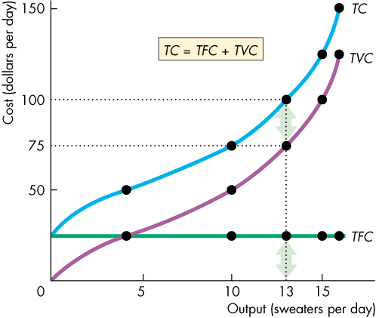
Total Cost Curve

Total fixed cost is the same at each output level (always a horizontal line)

Total variable cost increases as output increases (always increasing shaped curve) - > it first increases at decreasing rate but at a certain point it increases at an increase rate

Total cost, which is the sum of TFC and TVC as output increases (always increasing shaped curve, same as total variable cost curve). The Gap between TC and TVC on a graph is TFC

Creating the TVC

TVC represents the relationship between output and cost. The TVC curve gets its shape from the TP curve. The TVC curve becomes less steep at low output levels and steeper at high output levels.

To make it however, replace the quantity of labour on the x-axis with cost. Then redraw the graph with cost on the y-axis and output on the x-axis, and you’ve got the TVC curve.

Marginal Cost

Marginal cost (MC) is the change in total cost (new minus old) that results from a one-unit change in total product. Over the output range with increasing marginal returns, marginal cost falls as output increases. Over the output range with diminishing marginal returns, marginal cost rises as output increases. Has a U-shaped graph

Marginal product has an inverse relationship with Marginal cost

It is calculated as the change in total cost/ the change in quantity

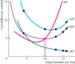
Average Cost

Average cost (per unit cost calculated by dividing Total cost by Quantity) measures can be derived from each of the total cost measures:

• Average fixed cost (AFC) is total fixed cost per unit of output (TFC divided by Quantity) - > not depend on quantity produced (always stays the same)

• Average variable cost (AVC) is total variable cost per unit of output (TVC divided by Quantity)

• Average total cost (ATC) is total cost per unit of output (ATC = AFC + AVC)

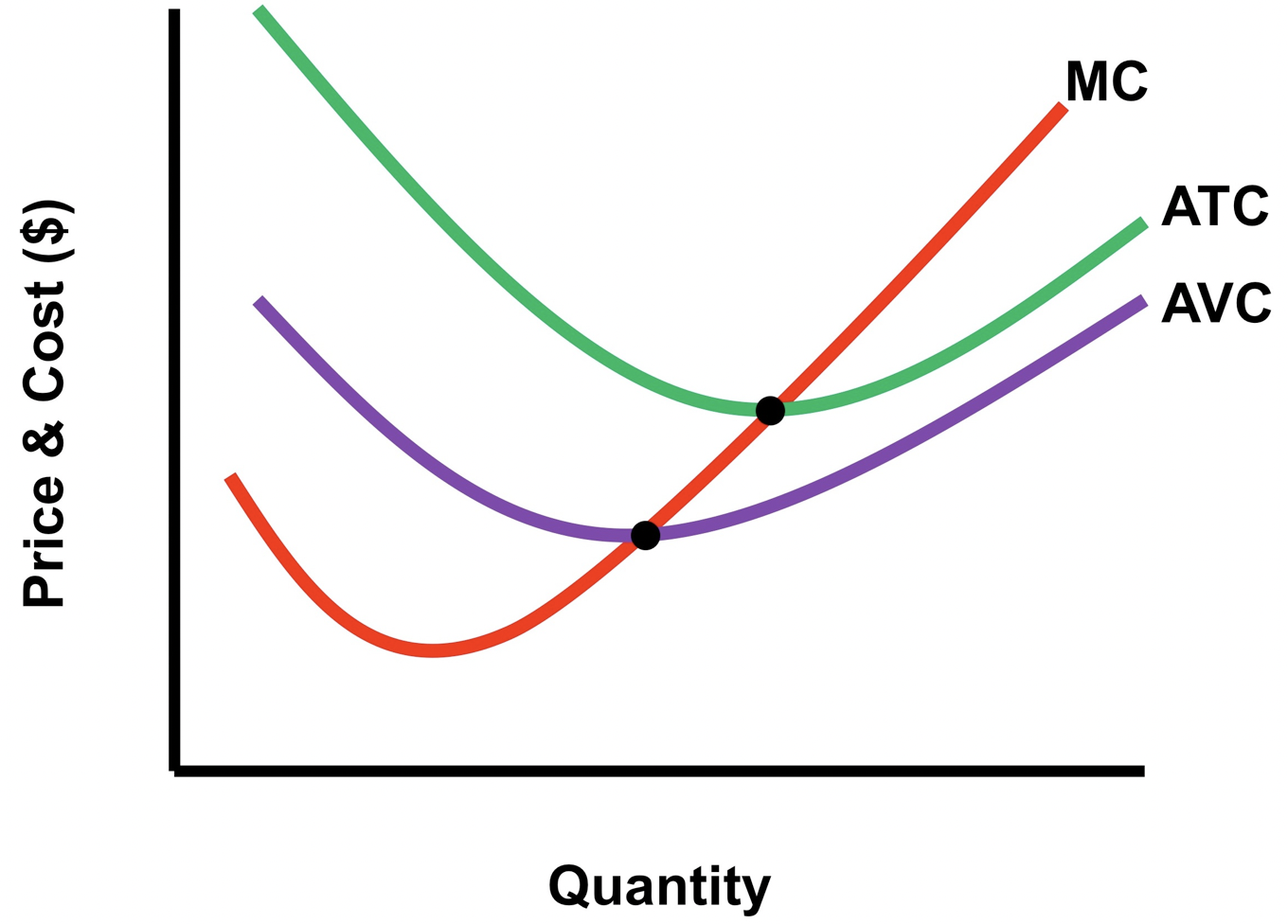
Average Cost Curves

The AFC curve shows that average fixed cost falls as output increases (always down word sloping but never touches x axis)

The AVC curve is U-shaped but slightly to the left. As output increases, average variable cost falls to a minimum and then increases.

The ATC curve is U-shaped but slightly to the right (same general shape as AVC). The outputs over which AVC/ATC is falling/ decreasing, MC is below AVC/ATC. The outputs over which AVC/ATC is rising/ increase, MC is above AVC/ATC. The output at which AVC/ATC is at the minimum, MC equals AVC.

Average Cost Curves Image

Why are the ATC and AVC U – Shaped?

Initially, MP exceeds AP, which brings rising AP and falling AVC.
Eventually, MP falls below AP, which brings falling AP and rising AVC.

The U-shape of the ATC curve arises from the influence of two opposing forces:

1. Spreading total fixed cost over a larger output—AFC curve slopes downward (they decrease) as output increases.
2. Eventually diminishing returns—the AVC curve slopes upward and AVC increases more quickly than AFC is decreasing so ATC increases and is upward sloping

*at higher output level, cost increases and lower output level, cost decreases

Relationship between MC, MP and AVC, AP

Importnat

Shifts in the Cost Curves

The position of a firm’s cost curves depends on two factors:
§ Technology
§ Prices of factors of production

Technology

An increase in productivity shifts the product curves upward and the cost curves downward.

If a technological advance results in the firm using more capital and less labor, fixed costs increase and variable costs decrease. In this case, average total cost increases at low output levels and decreases at high output levels

Prices of Factors of Production

An increase in the price of a factor of production increases costs and shifts the cost curves.

An increase in a fixed cost shifts the total cost (TC) and average total cost (ATC ) curves upward (increase) but does not shift the marginal cost (MC ) curve. An increase in a variable cost shifts the total cost (TC), average total cost (ATC ), and marginal cost (MC ) curves upward.

The Production Function

The behavior of long-run cost depends upon the firm’s production function.

The firm’s production function is the relationship between the maximum output attainable and the quantities of both capital and labor.

In the long run, all inputs are variable, and all costs are variable

Firms Production Function

As the size of the plant increases, the output that a given quantity of labor can produce increases.

But for each plant, as the quantity of labour increases, diminishing returns occur.

Long Run Cost

The average cost of producing a given output varies and depends on the firm’s plant.

The firm has 4 different plants: 1, 2, 3, or 4 machines

Each plant has a short-run ATC curve

MP and TP and MC and TC curves

*

MC and AVC and ATC Curves

*

.

]\.

Long Run Average Cost Curve

The long-run average cost curve or plant or enveloped curve is the relationship between the lowest attainable average total cost and output when both the plant and labour are varied.

The long-run average cost curve is a planning curve that tells the firm the plant that minimizes the cost of producing a given output range.

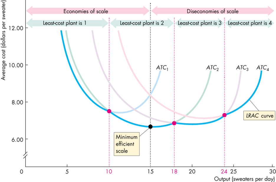
Long Run Average Cost Curve Illustration

*A part of short run (lowest cost) will be part of the long run curve

Long Run can be divided into three scales

Economies of scale are features of a firm’s technology that lead to falling/ decreasing long-run average cost as output increases (doubling of costs, produces more than double output)

Diseconomies of scale are features of a firm’s technology that lead to rising/increasing long-run average cost as output increases. (doubling of costs produces less than double output)

Constant returns to scale are features of a firm’s technology that lead to constant long-run average cost as output increases (where economics of scale and diseconomies scales intersect)

Minimum Efficient Scale

Minimum efficient scale is the smallest quantity of output at which the long-run average cost reaches its lowest level.

If the long-run average cost curve is U-shaped, the minimum point identifies the minimum efficient scale output level.