Working Capital management and short-term finance

Chapter 17

Objective of short-term financial management

Keep investment in cash and short-term assets as low as possible while skill keeping the firm operating efficiently and effectively.

Reasons for holding cash

3 motives for liquidity: Speculative motive, precautionary motive and transaction motive.

Speculative motive

the need to hold cash to take advantage of additional investment opportunties, such as bargain purchases might arise, favorable exchange rates, attractive interest rates

Precautionary motive

the need to hold cash as a safety margin to act as a financial reserve.

Transaction motive

the need to hold cash to satisfy nromal disbursement and collection activities associated with a firms ongoing operations: paying bills, salaries, trade debts, dividends.

Cash collected from sales of assets and new financing, inflows (collections) and outflows (disbursements) aren’t synchronized and some level of holdings needed to serve as buffer

Compensating balances

another reason to hold cash, cash balances kept at banks to compensate for banking services the firm recieves. Minimum compensating balance requirement may impose lower limit on level of cash a firm holds.

Costs of holding cash 

Cash held in excess of necessary minimum incurs opportunity cost - interest income that could be earned in next best use like investment in marketable securities. 

Why hold? cash balance needs to be maintained to provide liquidity neccesary for transaction needs - paying bills. If too small = may run out of cash. 

Determine appropriate cash balance by weighing benefits of holding against the costs. 

Distinction between Cash management VS Liquidity management

Cash m - closely related to optimizing mechanisms for collecting and distributing cash.

Liquidity m - concerns optimal quantity of liquid assets a firm should have on hand.

Managing short-term capital has specialists focus on

1. Liquidity management - manage cashflow and optimize efficiency through maintaining cash balances through cycle of short-term deficit and surplus positions.

2. Credit management - treasury responsible for designing firms optimal trade credit policy, use credit instruments for short-term financing needs.

3. Inventory management - if inventory/raw materials significant component to current assets, treasury will concern with impact on liquidity and ensure optimal inventory control systems in place.

4. Risk management

5. Advisory - provide financial advisory services to corporate management due to number of accountants and financially literate staff in treasury team.

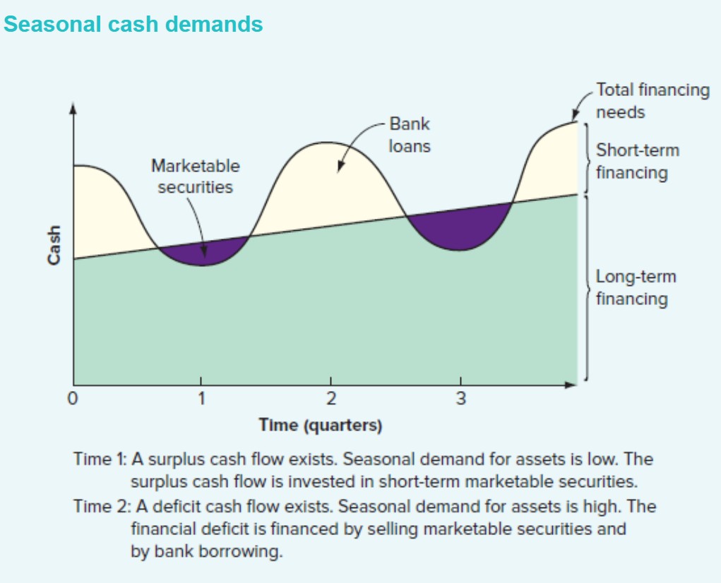
Seasonal or Cyclical activities in temporary cash surpluses 

some have predictable cash flow pattern, surplus cashflows part of the yr and deficit cashflow rest of the yr e.g. gazebos and bbqs are seasonal cash influenced by the weather. 

Firms like this buy marketable securities when deficits occur and bank loans to meet temporary financing needs 

Planned or possible expenditures in temporary cash surpluses

Firms frequently accumulate temporary investments in marketable securities to provide cash for plant construction programme, dividend payment or other large expenditure.

So firm may issue bonds and shares before cash is needed, investing proceeds in short-term marketable securities and then selling securities to finance expenditures.

Face possibility of having to make large cash outlay like possibility of losing a large lawsuit, may build up cash surpluses against such contingency.

Sources of short-term finance 

Liquidity management requires firm to dynamically manage liquidity so short-term fluctuations of cash and inventory are smoothed overtime. Can’t use volatility as creates risk of liquidity crunch unable to pay creditors or purchase inventory.

With temporary surplus cash balances, will want to invest it in very short-term money market instruments. With temporary deficit cash balance, want to draw on short-term financing offset the liquidity shortage. 

main sources: bank overdrafts, short-term loans, trade credit, short-term leases. 

Bank overdrafts

Allow firm to temporarily borrow from bank through current account. Once set up, can be used to smooth out short-term volatility in firms cash flow.

Provides flexibility in cash management at relatively low cost.

Commitment fee normally required when initially set up, annual fee for service. Overdraft limit agreed when using it so charged interest on daily basis for amount overdrawn

Short-term loan

For a set period and normal lender is the bank. Funds are released immediately and contracted payments are required over the life of the loan.

Both overdraft and short loan provide funding for short periods, short-term loan is for purchasing assets whilst overdraft is for smooth cashflow volatility from day-to-day trading.

Firms with both have maximum flexibility in cashflow management.

Short-term leases 

contractual agreement between lessee and lessor, establishing that lessee has right to use an asset and in return must make periodic payments to lessor, owner of asset. Either a manufacturer or independent leasing company, if independent then must buy asset from a manufacturer. 

Concern for the use of the asset, not for who owns the asset, lease contract allows asset to be used without ownership. Alternative is user to buy asset and involves alternative financing arrangements.

2 lease types: operating and financial leases.

Operating leases

Lessee recieved an operator along with the equipment.

Has several characteristics:

1. usually not fully amortized, payments required under the terms of the lease dont cover full cost of the asset for the lessor because life of oeprating lease is usually less than economic life of asset, so lessor expects to recover costs of assets by renewing the lease or selling asset for its residual value.

2. require lessor to maintain and insure the leased assets

3. gives lessee right to cancel lease contract before expiration date, if they cancel, lessee must return equipment to lessor. Value of cancellation clause depends on whether future technological or economic conditions are likely to make value of asset to lessee less than value of future lease payments under lease.

Financial leases

opposite to operating leases

1. dont provide for maintenance or service by lessor

2. fully amortized

3. lessee usually has right to renew lease on expiration

4. cant be cancelled, must make all payments or face risk of bankruptcy.

due to this, lease provides alternative method of financing purchase.

Investing idle cash 

Temporary cash surplus means they can invest in short-term securities. Market for short-term financial assets is money market, the maturity for these traded in money markets is 1 yr or less. Most manage their own sort-term financial assets, carrying out transactions through banks and dealers. Some large and small firms use money market mutual funds.

These funds invest in short-term financial assets for a management fee - compensation for the professional expertise and diversification provided by the fund manager. 

Among money markets, some specialise in corporate customers. Some banks offer arrangements in which bank takes all excess avaliable funds at close of each business day and invests them for the firm. 

money market instruments in 3 categories: interest-bearing instruments, discount info, derivatives. 

Interest-bearing instruments

Money market deposits - loan between banks, ranges from overnight to up to 12 months. Money market deposits are either fixed (interest rate/term decided at the beginning of contract or call (determined by benchmark rate/term can be shortened if prior notice given)

Certificates of Deposit (CD) - very short-term loan from companies with excess cash to a bank, has specified interest rate and tern. Negociable certificates of deposit can be sold before the instruments expiry date whereas a non-negociable certificate of deposit cant be traded and must be held to maturity. Like money market deposits except that the former is a loan by a company to a bank instead of between banks.

Repurchase agreements (Repo) - Firm will sell a security to another firm and simultaneously agrees to buy back in the future at higher price. Difference between sale price and subsequent purchase price is equivilant to interest e.g. government treasury bills or other low-risk short-term securities

Discount instruments

Zero-coupon debt securities with very short life of less than 12 months.

Treasury bills - short-term government debt securities, maturity ranges from 1 to 12 months.

Commericial paper - corporate equivilent of treasury bills, up to 12 months, most common maturity being 1 or 3 months. Only largest companies can issue commercial paper and instruments always unsecured.

Bankers acceptances - used by importers/exporters in countries where they dont have strong corporate presence. Company must firm set up bankers acceptance in facility with bank and issue discount instruments against facility. Bankers acceptance have maturity and sell at discount. Characteristic of bankers acceptance is bank guarantees payment and credit risk is lower than it otherwise may be. Borrowing firm pays the bank any money owed. Have less than 12 months maturity.

Derivative instruments 

1. Forwards - bespoke agreemet between 2 firms to exchange an asset (like cash) for set price at specified date in future.

2. Futures - standardised exchange-traded forward contract. Asset characteristics, asset quantitiy, price and contract maturity are standardised, future contracts can be traded on an exchange.

3. Options - Contract that gives holder the right but not obligation to buy or sell asset for set price at or before a specified date in the future. Option contracts may be bespoke or exchange traded. 

Target cash balance

A firms desired cash level determined by the trade-offs between carrying costs and shortage costs

Adjustment costs

the costs associated with holding too little cash - shortage costs

Determining target cash balance 

If firm has flexible working capital policy, can probably maintain marketable securities portfolio. Adjustment costs will be the trading costs associated with buying/selling securities. Cash management would be moving money in/out of marketable securities. 

If restrictive working capital policy, probsbly borrow in short term to meet cash shortages, cost would be interest and other expenses with arranging a loan. 

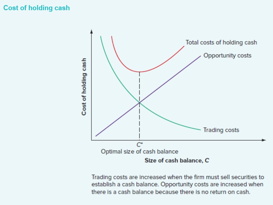
Basic idea of holding cash

For a flexible firm. If they keep cash holdings too low, find running out of cash more than desirable, so selling marketable securities more frequently than if cash balance was higher (possibly buying later to replace those sold). So trading costs will be high when cash balance is small, the costs fall as cash balance goes larger.

Opportunity costs of holding cash are low if firm holds little cash, costs increase as cash holdings increase as firm is giving up more interest that could be earned.

Total costs occur where the 2 individual cost curves cross at point C*. Where opportunity and trading costs are equal. This represents the target cash balance, the point firms should try to find.

The BAT model

This model can be used to establish target cash balance. Useful in illustrating factors in cash management and current asset management. BAT is simplest and stripped-down model for determining optimal cash position. Weakness of assuming steady, certain cash outflows. 

E.g. Start week 0 with cash balance of C = £1.12 million. Each week outflow exceed inflows by £600,000. As result, cash balance drop to zero at the end of week 2. Average cash balance beginnings balance (£1.2 million) + ending balance (£0) divided by 2 = £600,000 over 2 week period. End of 2 week period, replenish cash by depositing another £1.2 million. Cash balance declines by £600,000 per week. 

Assume net cash outflow is the same everyday and known with certainty. 

If C were set higher, £2.4 million, cash would last 4 weeks before firm would have to sell marketable securities but firms average cash balance woud increase to £1.2 million (from £600,000). If C set at £600,000, cash would run out in 1 week and replenish cash more frequently, average cash balance falls to £300,000. 

Because transaction costs must be incurred whenever cash is replenished (e.g. brokerage costs of selling marketable securities), establishing large initial balances will lower trading costs connected with cash management. Larger average cash balance = greater opportunity cost (return that could be earned on marketable securities).

F = Fixed cost of making a securities trade to replenish cash

T = total amount of new cash needed for transaction purposes over relevant planning period

R = Opportunity cost of holding cash, interest rate on marketable securities. 

Helps determine total costs of any cash balance policy and then optimal cash balance policy. 

The Opportunity costs

Need to find out how much interest forgone to calculate this.

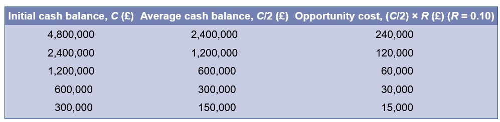
Total opportunity costs of cash balances are equal to average cash balance x interest rate.

Opportunity costs = (C/2) x R

E.g. £1.2 million initial cash balance, average is £600,000 (C/2), Interest could earn on this is 10% is £60,000, this is what firm gives up with this strategy. Opportunity costs increase as initial (average) cash balance rises.

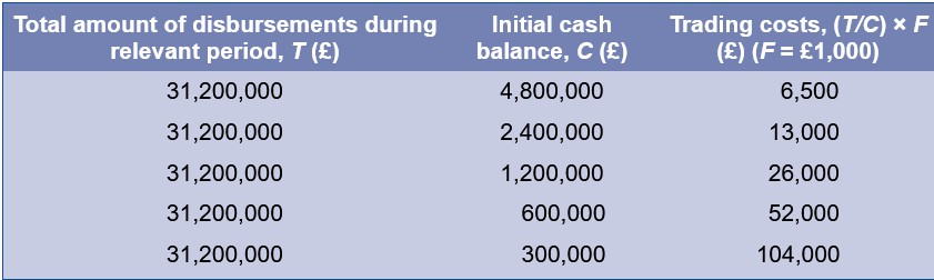
Trading costs

Need to know how many times firm will have to sell marketable securities during the year to calculate this.

Cash disbursed during the year (£600,000 per week) so T = £600,000 × 52 weeks = £31.2 million. If initial cash balance set at C = £1.2 million: £31.2 million/1.2 million = 26 times per year x F pounds cost (£1,000) = £26,000 Trading costs

Trading costs = (T/C) x F

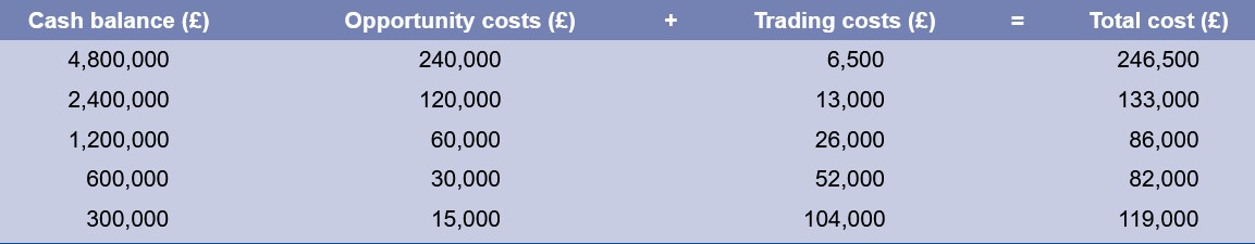
The Total cost 

Calculate by adding opportunity and trading costs together

Total cost = (C/2) x R + (T/C) x F

Total costs start at almost £250,000 and declines to £82,000 before rising again. 

£600,000 cash balance results in lowest total cost of possibilities presented £82,000

Optimal balance is between £300,000 and £1.2 million. Use trial and error to find optimal balance.

Optimal size of cash balance (C*) occurs where 2 lines cross. This is where opportunity cost and trading costs are equal: (C*) x R = (T/C*) x F

To solve C*: C* = √(2T x F)/ R Which is optimal initial cash balance 

C* = √(2 x £31.200,000 × 1,000)/ 0.10 = £789,937 leading to optimal cash level of £78,994 which does increase as move in either direction 

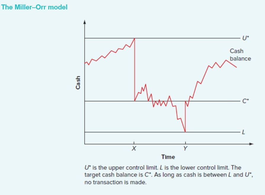
Miller-ORR model (general approach)

Designed to deal with cahs inflows/outflows that fluctuate randomly day-to-day. Concentrates on cash balance. Assumes balance fluctuates randomly and average change is zero.

Operates in terms of upper limit (U*) and lower limit (L) to amount og cash and target cash balance (C*). Firm allows cash balance to ander around between lower/ upper limits, as long cash balance is between U* and L, nothing happens.

When cash balance reaches upper (U*), the firm moves U* - C* cash out of the account into marketable securities. This moves cash balance down to C*.

If cash balance falls to lower limit (L), firm will sell C* - L worth of securities and deposit cash in the account, takes the cash balance up to C*.

Using the Miller-Orr model 

Set lower limit (L). This defines a safety stock, where its set depends on how much risk of cash shortfall firm is willing to tolerate. Alternatively, minimum might just equal required compensating balance.

Depends on trading and opportunity costs. Cost per transaction of buying and selling marketable securities F, summed to be fixed, opportunity cost of holding cash R, interest rate per period on marketable securities.

σ2 is the variance of the net cash flow per period. Can be anything like a day or week, as long as interest rate and variance are based on same length of time.

Given L, set by the firm, Miller show cash balance target C* and upper limit U* that minimise costs of holding cash: C* = L + (3/4 x F x σ2/ R) ^1/3 U* = 3 x C* - 2 x L

Average cash balance in Miller = (4 x C* - L)/ 3

If F = £10, interest rate is 1% per month, standard deviation of monthly net cashflows is £200, variance of monthly net cash flow is:

σ2 = £200² = £40,000

Assume minimum cash balance of L = £100, calculate cash balance target C*:

C* = £100 + (3/4 × 10 × 40,000/ 0.01)^1/3 = £411

The upper limit U* = 3 x £411 - 2 × 100 = £1,033

Average cash balance = (4 x £411 - 100)/ 3 = £515

Implications of BAT and Miller-Orr models 

Differ in complexity but similar implications

1. greater the interest rate, lower the target cash balance

2. greater the order cost, higher the target balance

Advantage of Miller is improves our understanding of problem of cash management considering effect of uncertainty, measured by variation in net cash inflows. 

Miller shows greater uncertainty (higher σ2 ) means greater difference between target balance and minimum balance. Greater uncertainty is, higher the upper limit and average cash balance.

Other factors influencing target cash balance

Assume cash is invested in marketable securities like treasury bills. Firm obtains cash by selling these securities. Another alternative is to borrow cash, it introduces additional considerations to cash management:

1. borrowing likely more expensive than selling marketable securities, because interest rate is likely to be higher.

2. Need to borrow will depend on managements desire to hold low cash balances, firm more likely to borrow to cover unexpected cash outflow with greater cash flow variability and lower investment in maketable securities.

For larger firms, trading costs of buying and selling securities are small when compared with the opportunity costs of holding cash. E.g. have cash not needed for 24 hrs, invest it or leave it?

If investing at annualized rate of 7.57% per yr, daily rate is about 0.02%, daily return earned on £1 million is 0.0002 x £1 million = £200. Order cost will be much less than this, so large firm will buy and sell securities very often before it will leave substantial amounts of cash idle.

Credit and recieveables

Granting credit is making an investment in a customer tied to sale of product/service. Used as a way to stimulate sales, costs associated arent trivial. Chance customer wont pay. Firm has to bear costs of carrying recieveables. Decision thus involves a trade-off between the benefits of increased sales and costs of granting credit.

Accounting perspective, credit granted means trade recieveable is created. To consumers is called consumer credit. 1/6 of all assets are in form of trade recieveable, so major investment of financial resources by businesses.

Components of credit policy 

Firm decides to grant credit to its customers, then must establish procedures for extending credit and collecting. In particular the firm will have to deal with components of credit policies. 

Terms of sale

the conditions under which a firm sells its goods and services for cash or credit.

If firm does grant credit to a customer, terms of sale will specify the credit period, cash and discount period and type of credit instrument

Credit analysis

The process of determining the probability that customers wont pay

Firm uses a number of devices and procedures to determine the probability that customers wont pay.

Collection policy 

the procedures followed by a firm in collecting trade receivables.

Investment in recieveables

Depends on amount of credit sales and average collection period. If average collection period is 30 days, then given time there will be 30 days worth of sales outstanding.

If credit sales run £1000 per day, firm trade recievabels will equal to 30 days x £1000 per day = £3000 on average

Trade recieveables = Average daily sales x ACP

Investment depends on factors that influence credit sales and collections.

Terms of the sale 

1. period for which credit is granted (credit period)

2. The cash discount and discount period

3. The type of credit instrument

Terms of sale are fairly standard but varies across industries. Some are archaic dating to previous centuries. 

The basic form terms of sale

Take the discount off incoice price if you pay in this many days, otherwise pay the full invoice in this many days

E.g. 2/10, net 60 are common. Means customers have 60 days from invoice date to pay the full amount, however if payment made within 10 days, a 2% cash discount can be taken.

Buyer places order for £1000 assuming terms of sale are 2/10 Net 60. Buyer has option of paying £1000 x (1-0.02) = £980 in 10 days, or pay full £1000 in 60 days.

If terms stated as just net 30, customer has 30 days from invoice date to pay entire £1000, no discount offered for early payment.

5.10 net 45 means take 5% from full price if paying within 10 days or else pay in full in 45 days

Credit period

the length of time for which credit is granted, varies per industry, almost always 30 to 120 days. If cash discount offered, then has net credit period and cash discount period.

Net credit period - length of time customer has to pay.

Cash discount period - time during which the discount is avaliable

E.g. 2/10 net 30 = net credit period 30 days and cash discount period 10 days

The invoice date 

beginning of the credit period

Invoice - a bill for goods or services provided by the seller to the purchaser. For individual items invoice date usually the shipping date or billing date, not date where buyer recieved goods or the bill. 

Terms of sale might be ROG (receipt of goods) where credit period starts when customer recieves order, might be used if they are in a remote loaction. 

EOM (end of the month) dating have all sales made during a particular month assumed at the end of the month. Useful when buyer makes purchase throughout the month, but seller bills only once a month. 

E.g. 2/10th EOM buyer takes 2% discount if payment is made by the 10th of the month. Sometimes end of the month is 25th day, MOM (Middle of the month)

Seasonal dating used to encourage sales of seasonal products during off-season, product sold primarily in the summer can be shipped in Jan with credit terms of 2/10 net 30, but invoice might date 1 May so credit period begins that time, encourages buyers to order early. 

Length of the credit period

Buyers inventory period and operating cycle influence this. All else equal, the shorter these are, shorter the credit period will be.

Operating cycle has 2 components: inventory period - time it takes buyer to acquire inventory, process it and sell it. Recieveables period - time it takes buyer to collect on sale. Credit we offer is the buyers payable period.

Extending credit, we finance portion of buyers operating cycle = shorten buyers cash cycle. If our credit period exceeds their inventory period, we are financing the buyers inventory purhcases and part of their recieveables.

If credit period exceeds buyers operating cycle, are effectively providing financing for aspects of our customers business beyond immediate purchase/sale of merch. Reason buyer effectively has a loan from us even after merch is resold, buyer can use credit for other purposes. So length of buyers operating cycle is cited as appropriate upper limit to the credit period.

Other factors influencing credit period

Perishability and collateral value: Perishable items have rapid turnover and low collateral value. Credit periods are shorter for such goods. E.g, a food wholesaler selling fresh fruit and produce might use net 7 days. Alternatively, jewellery might be sold for 5/30, net 4 months.

Consumer demand: Products that are well established have more rapid turnover. Newer or slow-moving products will have longer credit periods to entice buyers. Sellers may choose to extend much longer credit periods for off-season sales (when customer demand is low).

Cost, profitability and standardization: Relatively inexpensive goods have shorter credit periods. The same for standardized goods and raw materials. These all have lower mark-ups and higher turnover rates, both of which lead to shorter credit periods. However, there are exceptions. E.g. Car dealers pay for the vehicles as they are received.

Credit risk: The greater the credit risk of the buyer, the shorter the credit period is likely to be (if credit is granted at all).

Size of the account: If an account is small, the credit period may be shorter because small accounts cost more to manage, and the customers are less important.

Competition: When the seller is in a highly competitive market, longer credit periods may be offered as a way of attracting customers.

Customer type: A single seller might offer different credit terms to different buyers. E.g. food wholesaler might supply groceries, bakeries and restaurants. Each group would probably have different credit terms. More generally, sellers often have both wholesale and retail customers, and they frequently quote different terms to the two types.

Cash discounts 

a discount given to induce prompt payment. Also, sales discount., part of terms of sale. 

Offered to speed up the collection of receivables. This will have the effect of reducing the amount of credit being offered, and the firm must trade this off against the cost of the discount.

Cash discount offered means credit is free during discount period, buyer pays for credit after discount expires.

E.g. 2/10 net 30, buyer pays in 10 days for possible use of free credit or pays in 30 days for longest use of money in exchange of giving up the discount, giving it up means buyer gets 30 - 10 = 20 days credit. 

Another reason is a way of charging higher prices to customers that have had credit extended to them. Cash discounts are a convenient way of charging for the credit granted to customers.

Cost of the credit

Even small discounts provide an incentive as the implicit interest rate can be high.

E.g. order is £1000, buyer can pay £980 in 10 days or wait another 20 days and pay £1000. Buyer os borrowing £980 for 20 days and buyer pays £20 interest on loan.

The interest is ordinary discount interest, with £20 interest on borrowed £980, rate is £20/980 = 2.0408%. This is low but its the rate per 20 day period. 365/20 = 18.25 in a year, so not taking the discount means buyer pays EAR of 1.020408^18.25 - 1 = 44.6%

Buyers view this as expensive. As the interest is high here, seller may not benefit from early payment, ignoring the discount would help the seller.

Trade discounts and cash discount + ACP

Sometimes discounts arent incentives for early payment but a trade discount, discount given to some type of buyer E.g. 2/10th EOM terms, buyer takes 2% discount if invoice is paid by 10th, but bill considered due on 10th, overdue after that. So credit period and discount period are the same just without the reward of paying early.

Encouraging customers to pay early will shorten the recieveables period and all other things being equal, reduce firms investment in recieveables. E.g. firm has terms of net 30, average collection period (ACP) of 30 days. Offer terms of 2/10 net 30, then 50% customers pay in 10 days, remaining customers have advantage of 30 days to pay. What will new ACP be?

Annual sales are £15 million before discounts, if half take 10 days to pay and other hald take 30, average collection period will be: 0.50 × 10 days + 0.50 × 30 days = 20 days new ACP

Average daily sales are £15 million/365 = £41,096 per day, recieveables fall by £41,096 × 10 = £410,960

Credit instrument 

Evidence of indebtedness (customers owing money). Document of proof that someone has bough something on credit and must pay later E.g. Seller gives an invoice when goods are shipped, custoemr signs as evidence that goods have been recieved, record exchange in books. 

Open account

Most trade credit is on open account — the only credit document is the invoice. The customer receives the goods and the invoice and pays later. No formal loan contract. E.g. A business buys supplies and pays the invoice 30 days later.

Promissory note

A signed IOU promising payment in the future. Used when the order is large or when the seller wants added assurance of payment. E.g. Customer signs a promissory note agreeing to pay £10,000 in 30 days.

Commercial draft 

A document drawn up by the seller, telling the buyer to pay a set amount on a set date. It gets the buyer’s commitment before the goods arrive. 

2 types: Sight draft: Buyer must pay immediately. Time draft: Buyer pays later.

Trade Acceptance

A draft the buyer has accepted (agrees to pay later). Once the buyer signs/accepts it, it becomes a legally binding promise to pay. E.g. Buyer accepts a time draft for £5,000 due in 60 days → becomes a trade acceptance.

Bankers Acceptance

A draft guaranteed by a bank. The bank promises to pay, so its very safe and can be traded in money markets.

Conditional sales contract 

Seller keeps legal ownership of goods until the buyer completes the payment. Used for instalment plans; includes interest cost. 

E.g. Customer pays for equipment over 12 months; seller keeps ownership until fully paid

Factors in credit policy 

When a firm grants credit, these 5 things change:

1. Revenue effects — sales may increase.

2. Cost effects — costs occur immediately, but payment is delayed.

3. Cost of debt — firm must finance receivables.

4. Default risk — some customers won’t pay.

5. Cash discounts — some customers pay early to get a discount.

NPV of Granting Credit

Grant credit only if the Net Present Value (NPV) of doing so is positive. Granting credit must bring more benefit (extra profit) than cost (financing and risk)

NPV = PV of increased cashflow - cost of extra recieveables

Monthly profit before change and after

Monthly Cashflow = (P - v)Q 

P = price per unit,   Q = Current Quantity sold per month,  v = variable cost per unit,   Q* = Quantity sold under new policy,   r = monthly required return 

E.g. Monthly sales of P x Q (49 × 100) = £4,900, Variable costs each month is v x Q (20 × 100) = £2,000. 

Cashflow with old policy is (P - v)Q = (49 - 20) x 100 = £2,900

If they switch to net 30 days on sales, quanity sold will rise to Q* = 110. Monthly revenue increase to P x Q* and costs will be v x Q*.

New policy cashflow: (P-v)Q* = (49 - 20) x 110 = £290 

Incremental cashflow 

The difference between the new and old cash flows 

Incremental cash inflow = (P - v)(Q* - Q) 

E.g. (49 - 20) x (110 × 100) = £290 

Equal to gross profit per unit sold (P-v) x increase in sales (Q*-Q) 

Present value of future incremental cashflow is: PV = ((P-v)(Q*-Q))/ r 

E.g. (29 × 10) / 0.02 = £14,500 

Cost of switching credit policy

As quantity sold will rise from Q to Q*, need to produe Q* - Q more units at a cost of

v(Q*-Q)

E.g. 20 x (110 - 100) = £200

Sales collected this month under current policy (P x Q = 4,900) wont be collected.

New policy, sales made this month not collected until 30 days later.

Cost of switching = PQ + v(Q*-Q)

E.g. 4,900 + 200 = £5,100

NPV of switching policy

NPV of switching = -(PQ + v(Q*-Q) + ((P -v)(Q*-Q)) / r

Cost of switching is £5,100 and benefit per month is £290 for ever, at 2% per month, NPV is:

NPV: -£5,100 + 290/ 0.02 = -5,100 + 14,500 = £9,400

Positive number means switch to credit is profitable 

Break-even increase in sales

Calculate break-even by setting NPV in equation to zero and solving for (Q*-Q)

Q*-Q = PQ/ (P-v)(r - v)

E.g. Q* - Q = £4,900/ (29/0.02 - 20) = 3.43 units to be sold to break even

Tells us if switch is good idea as long as confident to sell at least these units per month

Optimal credit policy 

The level of credit a firm should offer 

Extra profit from extra sale = extra cost of offering more credit 

Give enough credit to boost sales but not so much that the cost of slow collection, bad debts and admin outweighs the benefits

Carrying costs of granting credit

Costs that increase when you offer more credit:

• Required return on receivables

  • Money tied up in credit could have earned interest elsewhere.

• Bad debt losses

  • More credit → more risk some customers won’t pay.

• Credit department costs

  • Staff, admin, systems to monitor receivables.

As credit becomes more relaxed (easy to get), these costs go up

Opportunity costs NOT granting credit 

These are the profit you lose by being too strict:

1. Lost sales (Q' – Q drops)

   • Customers may not buy if credit isn’t available.

   • Lower quantity sold = lower revenue.

2. Potentially lower prices

   • Firms sometimes charge higher prices only when credit is offered.

As credit becomes more restrictive, these opportunity costs go up

Total credit cost curve 

Total credit cost curve = Carrying Costs + Opportunity Costs.

If credit is too strict → low carrying costs but high opportunity costs
If credit is too loose → high carrying costs but low opportunity costs

There is a minimum point in the middle.

The minimum point = Optimal credit policy
This is where total costs are lowest and profit is maximised.

What influences a more liberal credit policy?

Firms are more likely to offer generous credit terms when they have:

1. Excess Capacity

• Extra unused production capacity

• More sales = spreads fixed costs better

• Credit boosts demand

2. Low Variable Costs

• If it’s cheap to produce each extra unit, the profit margin is bigger

• So increasing sales through credit is attractive

3. Repeat Customers

• Long-term customers → lower risk and predictable payments

• Bigger incentive to keep them happy with easier credit terms

Key insight 

Optimal credit policy is a balancing act:

• Offer enough credit to increase sales and profits

• But not so much that you create costly receivables, bad debts, or high admin expenses

The goal is to reach the level where:

Incremental Benefit = Incremental Cost

That point maximises profit.

Credit analysis

The process of deciding whether a customer should recieve credit

Requires:

1. Gathering information

2. Judge creditworthiness

NPV of Granting Credit to a One-time sale

NPV= −v+ (1- π)P​ / 1 + r

If customer buys one unit on credit at price of P per unit and its refused, customer wont make the purchase.

If credit is granted, then one month, the customer will pay up or default. The second event probability is π (percentage of customers who wont pay).

• v = variable cost

• π = default probability

• P= price

• r = monthly required return on recieveables

E.g. With 20% rate. NPV = -£20 + (1- π) x 49/1.02 = £18.43

Credit should be granted

Break-even default probability

Set NPV = 0

In granting credit to a new customer, firm risks its variable cost (v) but it stands to gain the full price (P). For a new customer, then, credit may be granted even if default probability is high.

NPV = 0 = -£20 + (1 - π ) x 49/1.02

1 - π = £20/49 × 1.02 = π = 58.4% max acceptable default probability for a new customer

Should extend credit, as long as there is a 1 - 0.584 = 41.6% chance or better of collecting. Explains why firms with higher mark-ups tend to have looser credit terms.

If returning, cash-paying customer wanted to switch to credit basis, analysis would be different and maximum acceptable default probability would be much lower.

Difference is, if we extend credit to returning customer, we risk total sales price (P), because this is what we collect if we dont extend credit, if we extend credit to new customer, we risk only variable cost.

Repeat customer business 

Value of one good customer: P-v/ r every month for ever 

NPV of granting credit: NPV = -v + (1-π ) P-v / r

A long-term customer is very valuable, so firms tolerate higher risk 

E.g. NPV = -20 + (1-π ) x (49-20)/ 0.02 

-20 + (1-π ) x 1450

Even if probability default is 90%: -20 + 0.10 × 1450 = £125

Extend credit unless default is a virtual certainty. Good customer is worth £1,450, however can afford quite a few defaults. 

Best outcome is extend credit to almost anyone. Possibility of repeat business needs consideration. Control the amount of credit initially offered to any one customer, so possible loss is limited. Amount can be increased in time. Best predictor of whether or not someone will pay in future is whether they paid in past or not. 

Average collection period (ACP)

Average time customers take to pay. ACP fluctuates but if rises unexpectedly, thats a warning sign. Means customers in general taking longer to pay or some percentage of trade recieveables are seriously overdue.

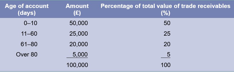
Ageing schedule

A table grouping recieveables by age. Shows how much money is owed and how late payments are.

Example Table:
0–10 days: £50,000
11–60 days: £25,000
…and so on.

E.g. have credit period of 60 days, then 25% of accounts are late, if its serious depends on anture of the firms collections and customers

Firms with seasonal sales will find the percentages on the ageing schedule changing during the year. E.g. if sales in the current month are very high, then total receivables will also increase sharply. This means that the older accounts, as a percentage of total receivables, become smaller and might appear less important. Some firms have refined the ageing schedule so that they have an idea of how it should change with peaks and valleys in their sales.

Collection effort 

A firm usually goes through the following sequence of procedures for customers whose payments are overdue:

It sends out a delinquency letter informing the customer of the past-due status of the account.

It makes a telephone call to the customer.

It employs a collection agency.

It takes legal action against the customer.

firm may refuse to grant additional credit to customers until arrears are cleared up. This may antagonize a normally good customer, which points to a potential conflict between the collections department and the sales department.

In probably the worst case, the customer files for bankruptcy. When this happens, the credit-granting firm is just another unsecured creditor. The firm can simply wait, or it can sell its receivable.

Types of inventory

• Raw materials

• Work-in-progress

• Finished goods

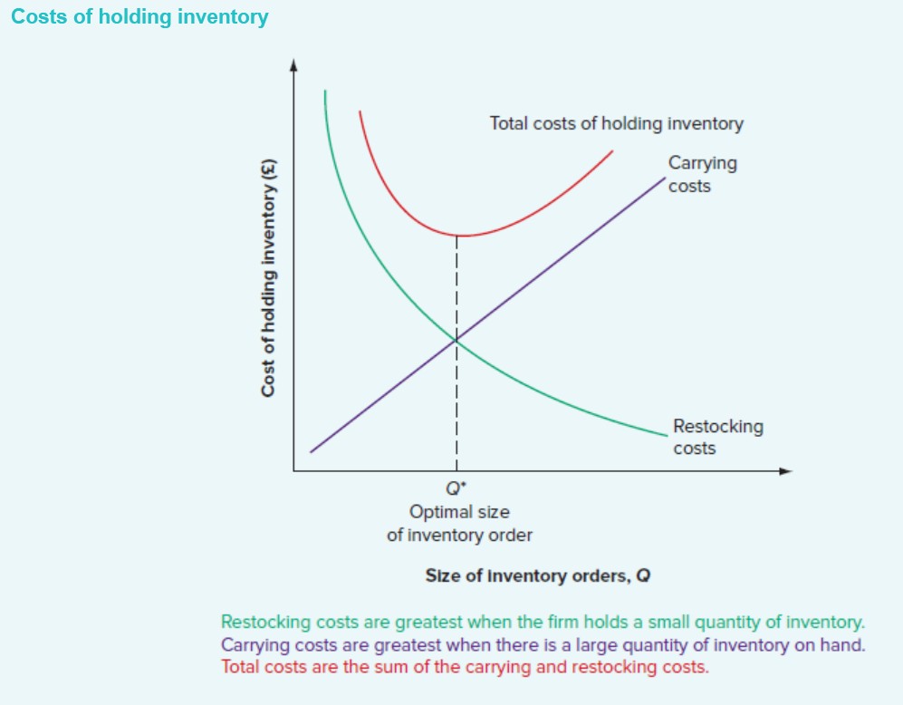
Inventory costs

Carrying Costs: (increase with more inventory)
Storage, insurance, obsolescence, capital cost.

Shortage Costs: (decrease with more inventory)
Lost sales, restocking cost, customer dissatisfaction.

Trade-off: more inventory means higher carrying costs

Less inventory means higher shortage costs. Optimal level is where total cost = lowest

Inventory management

both credit policy and inventory policy are used to drive sales, and the two must be co-ordinated to ensure that the process of acquiring inventory, selling it, and collecting on the sale proceeds smoothly.

Despite the size of a typical firm’s investment in inventories, the financial manager of a firm will not normally have primary control over inventory management. Instead, other functional areas such as purchasing, production and marketing will usually share decision-making authority regarding inventory.

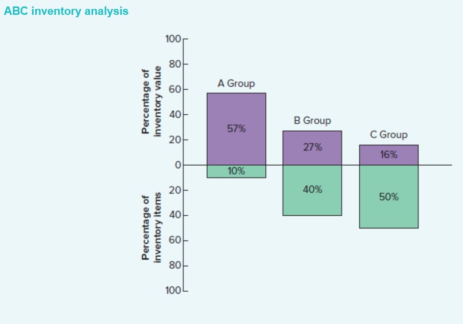
ABC inventory approach 

A simple way to classify inventory into importance categories.

Groups:

• A items

  • High value (≈ 50% of inventory value)

  • Low quantity (≈ 10% of items)

  • Monitored closely

• B items

  • Medium value, medium quantity

  • Normal control

• C items

  • Low value (nuts, bolts, cheap parts)

  • High quantity (≈ 70% of items)

  • Stocked in bulk

Purpose:
Focus attention on the items that matter financially (A items).

Economic order quantity (EOQ)

EOQ = order size (restocking quantity) that minimizes total inventory cost.

Key Assumptions

• Inventory is used at a steady rate

• When stock reaches zero → restock instantly

• Costs do NOT include cost of inventory itself

• Demand is known and constant

Established optimal inventory level

Mechanics of EOQ

Inventory starts at Q units → falls steadily to 0 → restocked to Q.

Average inventory = Q/2

Inventory-carrying costs rise and restocking costs decrease as invenotry levels increase. 

We assume that the firm’s inventory is sold off at a steady rate until it hits zero. At that point, the firm restocks its inventory back to some optimal level. E.g. starts out today with 3,600 units of a particular item in inventory. Annual sales of this item are 46,800 units, which is about 900 per week. If sells off 900 units of inventory each week, all the available inventory will be sold after 4 weeks, and will restock by ordering (or manufacturing) another 3,600 and start again. This selling and restocking process produces a sawtooth pattern for inventory holdings. On average, then, inventory is half of 3,600, or 1,800 units.

Carrying cost formula (CC)

Carrying cost = Q/2 x CC

Q = order quantity

CC = carrying cost per unit per year

E.g. Q = 3600 units and CC = £0.75

3600/ 2 × 0.75 = 1800 × 0.75 = £1350 per year

Restocking cost formula (shortage costs)

Restocking cost = F x (T/ Q)

• F = fixed cost per order

• T = annual demand

• Q = order quantity

E.g. T = 46,800 units, Q = 3,600, F = £50:

50 × (46800/ 3600) = 50×13 = £650 per year

Total inventory cost formula 

Total costs = Carrying costs x restocking costs

(Q/ 2) x CC + F x (T/ Q)

Goal is finding the value of Q, restocking quantity that minimizes the cost 

U-shaped where minimum point is where carrying costs = restocking costs 

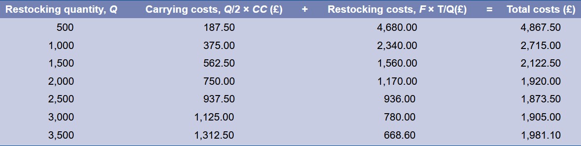
EOQ Formula

To minimise total cost, set Carrying Cost = Restocking cost

(Q*/ 2) x CC = F x (T/Q*)

Solve for Q* (EOQ): Q*² = √2T x F / CC

E.g. F = £50, T = 46,800, CC = £0.75

• Carrying Cost = Restocking Cost

• Total cost is minimised

• Company avoids too many small orders or big orders

Safety Stock (Minimum Inventory)

Extra inventory kept “just in case” to prevent stock-outs.

Impact:

• Raises average inventory

• Increases carrying cost

• Reduces risk of shortages

Graphically:
Inventory never drops to zero → a minimum level is always held.

Reorder Point

The inventory level at which a new order is placed.

Used because:

• Delivery takes time

• You don’t want to hit zero stock during the wait

Formula (simple version):

Reorder Point=Demand per day×Lead time

If safety stock is included:

Reorder Point = (d×L) + SS

• d = demand per day

• L = lead time in days

• SS = safety stock

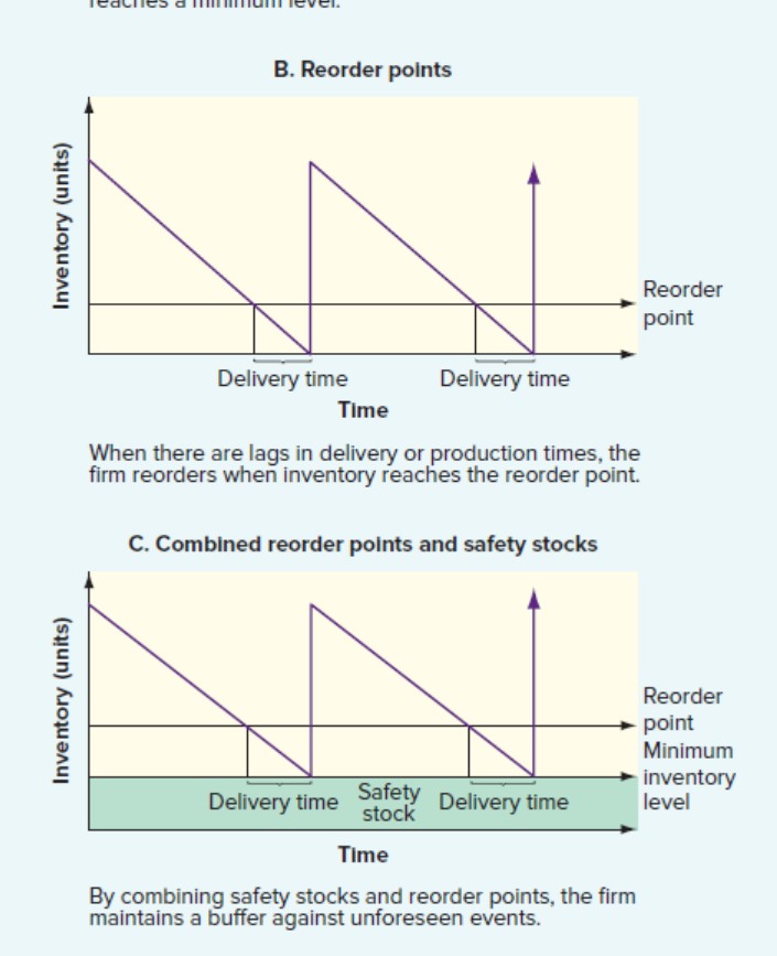
Combining safety stock and reorder point

This creates a generalised EOQ model:

• EOQ tells you how much to order

• Reorder point tells you when to order

• Safety stock tells you minimum level to protect against uncertainty

Managing Derived-Demand Inventories

Some inventory depends directly on production needs:

Examples:

• Car tyres depend on number of cars being built

• Bottles depend on number of drinks to be filled

These need planning systems, not simple EOQ.

Materials Requirements Planning (MRP)

Computer system that calculates exactly how much raw material and work-in-progress is needed to make the required finished goods.

Uses backward scheduling:

Finished goods → required components → required raw materials.

Used in industries with complex components (cars, electronics).

Just-In-Time (JIT) Inventory

Inventory arrives just when needed → inventory levels kept extremely low.

Key features:

• Frequent small deliveries

• Very high supplier coordination

• Used in Japanese manufacturing (Toyota)

Benefits:

• Lower carrying costs

• Less waste

• Faster production cycles

Downside:

• Vulnerable to supply chain delays

• Needs reliable suppliers

Kaban (part of JIT) - A signalling system (often a card) that tells suppliers to deliver more inventory.

Example:
A worker removes a bin of parts → card is sent to supplier → supplier sends replacement bin.

Summary: When Each Technique Is Used

ABC analysis

When some items are expensive and others cheap; prioritisation needed

EOQ	When demand is steady and predictable

Safety stock

When demand or delivery times are uncertain

Reorder point

When lead times must be considered

MRP	Complex products with many components

JIT	Highly efficient, reliable supply chain; minimise inventory