BA305 Midterm 2

Neural Networks definition

Artificial Neural Networks are flexible models used for classification, regression, and feature extraction.

Neural Networks inspiration

Mimics how neurons work in the brain by processing weighted inputs and firing signals.

Neural Networks applications

Used in areas like voice/image recognition, stock prediction, fraud detection, and self-driving cars.

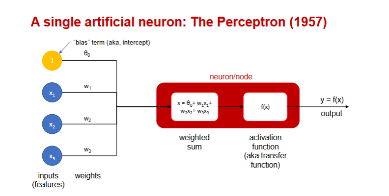
Perceptron structure

• Inputs (features)

• Weights assigned to each input

• Bias term (intercept)

• Activation function

• Output

Activation functions: sigmoid

smooth probability output restricted to [0,1]

Activation functions: ReLU

effective for deep learning. solves vanishing gradient problem. not differentiable at the point zero. f(x) = max{0, z}

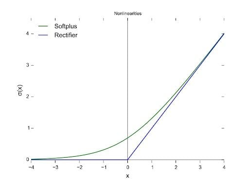
Activation functions: Step function

binary output

Activation functions: Tanh

scaled between -1 and 1

Layers of a NN:

• Input layer (features)

• Hidden layers (process data)

• Output layer (final prediction)

Input layer

takes the features.

Hidden layers:

processes the data.

Output layer

gives the final prediction.

Deep Learning

 Involves multiple hidden layers for enhanced complexity.

NN Optimization Techniques: Gradient Descent

Adjusts weights iteratively to minimize error.

NN Optimization Techniques: Backpropagation

Distributes error across layers to refine weights.

Overfitting in NNs is caused by:

Limited iterations

NN Overfitting Solution:

tracking validation error, cross-validation.

NN Data Requirements

significant computational power.

Tesla's Full Self-Driving (FSD)

Example of real-world NN implementation. Uses 48 neural networks trained with massive data and GPU hours.

Examples of NN business use cases

Consumer behavior prediction, fraud detection, and autonomous systems

NN advantages

• Good predictive ability 

• Can capture flexible/complicated relationships between outcome and predictors

NN Disadvantages

• Major danger is overfits in general

• A “black box” prediction machine, with no insight into relationships between predictors and outcome  

• Infinite architectures to choose from…virtually infinite design space

• Requires large amounts of data

• No variable-selection mechanism, need to exercise care in selecting variables  

• Heavy computational requirements if there are many variables (additional variables dramatically increase the number of weights to calculate

Logistic regression definition

Logistic Regression (LR) is an extension of linear regression designed for classification problems.

Linear regression vs logistic regression

Linear regression predicts continuous values, while logistic regression predicts probabilities that map to discrete categories.

Logistic Regression use cases

Used for binary classification (e.g., determining whether an event occurs or not).

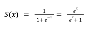
Sigmoid function

Ensures predictions remain between 0 and 1, making it ideal for probability modeling. y is not a target variable

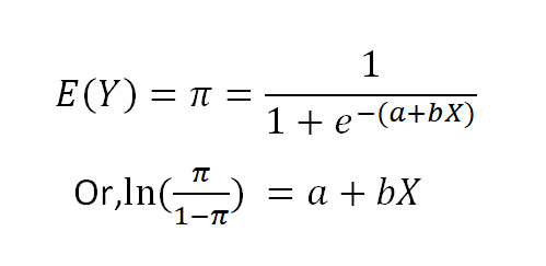
Logit Model

• Parameters:

  • 'a' Coefficient: Controls the probability curve shift.

  • 'b' Coefficient: Determines the steepness of the curve.

Logistic Regression optimization method

Instead of minimizing RMSE (like in linear regression), logistic regression maximizes log-likelihood, which is done automatically in Python.

Logistic Regression classification decision

• Converts probability outputs into categories using a cutoff threshold (e.g., default is 0.50).

• Cutoff can be adjusted to optimize accuracy, sensitivity, false positives, or cost of misclassification.

Logistic Regression Original Coefficient

Helps indicate direction of the relationship.

LogReg Exponentiated Coefficient (Odds Ratio):

Measures the magnitude of the relationship, how much odds change when the predictor variable increases by one unit.

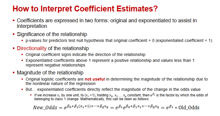
LogReg Exponentiated Coefficient Example

If odds ratio ( e^{b} = 1.114 ), a unit increase in the independent variable increases the odds of Y=1 by 11.4%.

LogReg Considerations: Multicollinearity

• Issue: Redundant predictors can cause unstable estimates.

• Solution: Remove redundant variables using feature selection or data reduction methods such as Principal Component Analysis (PCA).

LogReg Considerations: Overfitting

• Issue: Complex models may fit training data well but fail on validation data.

• Solution: Reduce variable complexity and always use separate training/validation datasets.

LogReg p-values

p-values for predictors test null hypothesis that original coefficient = 0 (exponentiated coefficient = 1)

NN strengths

 high predictive performance
 can capture complicated, “non-linear” relationships between variables

Perceptron

Some examples of activation functions

Neural network detailed description

A neural network consists of a layered, feedforward, fully connected network of perceptrons* or more advanced building blocks
 Multiple layers: Input, Hidden, Output
 Nodes (neurons)
 “Deep learning” refers to ~3+ hidden layers

NN basic idea

 Combine input information in a complex &
flexible neural network “model”
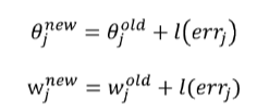
 Model “coefficients” are continually tweaked
computing gradients, in an iterative local
optimization process called backpropagation
 Backpropagation gets better the more iterations
you run (epochs)

NN preprocessing steps

 All features are required to be numerical
 Scale variables down, min-max, or standardization
 Decide what is appropriate based on the nature of the activation function!
 Categorical variables must be dummy coded

Iterative passes through network

At each iteration compare prediction to actual
 Various types of loss functions (like RMSE) can be used to measure error
 Error is propagated back and distributed to all the hidden nodes and used to update their weights
 l = constant between 0 and 1, reflects the “learning rate” or “weight decay parameter”

too small learning rate:

convergence extremely slow

too large learning rate:

faster learning, but may “overshoot” and fail to converge

NN Mapping the output:

E.g., in classification, output is between 0 and 1
 Classification: if probability exceeds the cutoff, classify as “1”, else “0”
 Prediction with metric output: Denormalization: the normalization needs to be inverted

NN Considerations: Hidden Layers

One hidden layer generally works well

NN Considerations: Number of nodes in hidden layers

More nodes capture complexity, but increase
chances of overfit

NN Considerations: Learning Rate

Low values:
 Downweights the new information from errors at each iteration
 Slows down learning, but reduces tendency to overfit to local structure

Learning rate: Allow the learning rate to change values as the training moves forward

 At the start of training, it should be initialized to a relatively large value to allow the network to quickly approach
the general neighborhood of the optimal solution
 When the network is beginning to approach convergence, the learning rate should gradually be reduced,
thereby avoiding overshooting the minimum

Logreg classification & cutoff process

Model produces an estimated probability of being a “1”, p(Y=1)
 Convert to a classification by establishing cutoff level
 If estimated prob. > cutoff, classify as “1”
 0.50 is standard initial choice of cutoff, but not necessarily the best one

Logreg cutoff considerations

 Maximize classification accuracy
 Maximize sensitivity (subject to min. level of specificity)
 Minimize false positives (subject to max. false negative rate)
 Minimize expected cost of misclassification (need to specify costs)

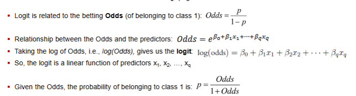
Logreg odds probability

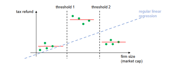
Decision tree definition

A popular ML method for prediction, like k-NN and Naïve Bayes, pioneered by Breiman et al. (1984). The output is not just a predicted result, ‘y=0’ or ‘y=1’, or a probability, p(y=1|x), but
also a set of general “rules” for why we arrived at the result

Decision trees vs K-NN

Remember for k-NN:
 Collect x={ income=65,000, family members = 1, credit card balance =1000}, then find neighbors, and
determine y:{“loan default”} class (but we don’t know anything more than that)
 But Trees are different: generate rules
 If x={ income>60,000, family members < 2, education < PhD}, then y={“loan accept”}=0 (and we know why)
 If x={ income<60,000, family members < 2, education > BS}, then y={“loan accept”}=1 (and we know why)

Decision Tree - CART

Decision trees also called Classification & Regression trees (CART)

Classification Trees: When the output represents a class, like y=‘spam’ or y=‘ham’, or y=0 or y=1

Regression Trees: When the output represents a continuous value, e.g., predicting house prices in a given area

CART trees inputs

In both cases, the inputs can be a mixture of categorical and numerical
 k-NN works best with numerical inputs but can accommodate some categorical as well
 Multinomial Naïve Bayes works only with categorical inputs
 Gaussian Naïve Bayes (which we did not see) works best with numerical inputs
 CART is more flexible

Multinomial NB

• Bayes' Theorem: The algorithm uses Bayes' theorem to calculate the probability of a class given a set of features. 

• Feature Independence: It assumes that the presence of one feature is independent of the presence of other features, given the class. 

• Multinomial Distribution: It models the likelihood of features using a multinomial distribution, which is appropriate for count data. 

• Prediction: The algorithm predicts the class with the highest posterior probability. 

Root Node

The first decision point that splits the dataset.

Decision Nodes (Internal Nodes)

Further splitting occurs based on feature values.

Leaf Nodes

Final classification or predicted value.

Majority Vote

The first step is identifying the most frequent class in the dataset.

Splitting

• The dataset is split using different features (e.g., "size" or "charges") to minimize classification errors.

• Example: Splitting by "charges" might yield a lower error rate than splitting by "size."

Stopping Criteria

The process stops when:

• A node has zero classification mistakes (pure leaf).

• There are no more features left to split on.

Error Rate

Measures the percentage of misclassified points.

Gini Impurity

Measures how mixed the classes are in a node.

Entropy

Determines the average number of yes/no questions needed for classification

Threshold Selection

Used for numerical inputs (e.g., "Size < 50" vs. "Size > 50")

Overfitting and Tree Pruning: Full Tree Issue

If grown indefinitely, trees overfit training data and perform poorly on unseen data.

Overfitting and Tree Pruning: Pruning Methods

• Limit tree depth.

• Set a minimum number of samples required in leaf nodes.

• Complexity penalty to reduce unnecessary splits.

Random Forests definition

An ensemble method that builds multiple Decision Trees using random sampling and predictor selection

Random Forests Steps

• Bootstrap sampling of training data.

• Random feature selection for each tree.

• Majority voting (classification) or averaging (regression) for final prediction

Random Forests Advantage

Improves accuracy while reducing overfitting

Ensemble methods

increase performance by providing several extensions to trees that combine results from multiple trees

Overfitting: Unstable Trees

Trees can also be unstable
 If 2 or more variables are of roughly equal importance, which
one CART chooses for the first split can depend on the initial
partition into training and validation
 A different partition into training/validation could lead to a
different initial split
 This can cascade down and produce a very different tree
from the first training/validation partition
 Solution is to try many different training/validation splits – k-
fold “cross validation” is going to be an important factor for
decision trees in general.

Some restrictions to limit tree growth for optimal accuracy

 Maximum tree depth (longest path between the root node and the leaf node).
 Minimum number of records in split nodes
 Minimum number of records in terminal node
 Minimum impurity increase needed to conduct a split on the next column

How to find optimal values for parameters

Use Grid or Randomized Search on training data, coupled with cross-validation
 Build multiple trees using different values for the parameters, using the training fold
 Measure accuracy on the holdout fold
 Choose tree with best performance
 Assess its performance on the validation, i.e., test data, not used at all to this point

Regression Trees - SSR

In every result “box” rather, than list the number of events “true, 1” vs “false, 0”, we instead compute the “average” value.

• At each box, for every possible threshold… add up the squared residuals

• The tree will (eventually) find the right splits

Regression Trees vs Linear Regression

For this type of data, linear regression underperforms (assuming right thresholds are chosen)