7: Production

Theory of the Firm

Explains how a firm makes cost-minimizing production decisions and how its cost varies with its output.

Production Technology, Cost Constraints, Input Choices

Three steps in understanding production decisions of firms:

Production Technology 

Describe how inputs can be transformed into outputs

Cost Constraints

Firms must take into account the prices of labor, capital, and other inputs

Input Choices

Given its production technology and the prices of labor, capital, and other inputs, the firm must choose how much of each input to use in producing its output.

very short run, short un, long run, very long run

Time Horizons

Very short run

all factors of production are fixed (e.g., on one particular day, a firm cannot employ more workers or buy more products to sell)

Short run 

one factor of production (e.g., capital) is fixed.

Long run

all factors of production of a firm are variable (eg, a firm can build a bigger factory).

Very long run

all factors of production are variable, and additional factors outside the control of the firm can change, e.g., technology, government policy. A period of several years.

production function

A __for any commodity is an equation, table, or graph showing the quantity that can be produced for each combination of alternative inputs

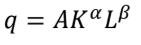
• Input-output relationship [q = f(K,L)]

• Production process as a “black box”

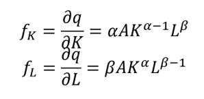
MP_k = fk = partial derivative of Q with respect to K

Marginal Physical Product (MP) formula

AP_k = Q/K

Average Product (AP) Formula 

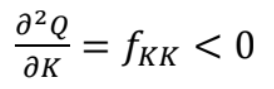
Law of Diminishing Marginal Returns

what formula is this:

positive

The APL curve usually rises at first, reaches a maximum, and

then falls, but it remains __ as long as the TP is positive.

zero, negative

The MPL curve also rises at first, reaches a maximum, and then declines. Notice that the MPL becomes__ when the TP is maximum and __when the TP begins to decline

law of diminishing returns

The falling portion of the MPL curve illustrates the__

increasing rate

Stage 1 of Production: TP – increasing @__

max

Stage 1 of Production: AP – increasing to __

max then falling

Stage 1 of Production: MP – increasing to__

decreasing rate

Stage 2 of Production: TP – increasing @ __

falling

Stage 2 of Production: AP –___

zero

Stage 2 of Production: MP – falling to __

max to falling

Stage 3 of Production: TP – from__

falling

Stage 3 of Production: AP – __

falling (negative)

Stage 3 of Production: MP –__

Marginal Products

Cobb-Douglas Production Function

Returns to Scale

Refers to the response of output when all inputs are increased simultaneously and proportionately. Given q = f(K, L)

degree of homogeneity of the production function

Let γ any constant factor by which L and K are increased

γ^hq = f(γK, γL)

Where h – __

alpha + beta = h

For Cobb-Douglas Production Function, RTS is just __

Isoquant

Locus of points, each point representing a combination of inputs which yields the same level of output

IQ that lies above and to the right of another represents higher levels of output, Negatively sloped, Never intersect, Convex to the origin

Characteristics of Isoquants

Isocost

Locus of points, each point representing a combination of inputs that a firm can purchase at the same time given its budget C = wL + rK

C = wL + rK

Constraint/Isocost formula

cost-minimizing choice of inputs

The point of tangency of the isoquant and the isocost line tells us the __, L and K.

Slope of the isocost = slope of the isoquant

Tangency Condition

-w/r

slope of isocost

-MRTS_LK

slope of isoquant

MPL/w = MPK/r

Equimarginal Principle Formula

equivalent amount of output

When cost is minimized, each dollar of input added to the production process will add an __.

Min C = rK + wL

Objective Function:

st q0 = f(K, L)

(Lagrange) Constraint:

Z = rK + wL + lamda[Q_0 − f(K, L)]

Lagrange equation:

Expansion Path

Locus of cost-minimizing tangencies, assuming fixed input prices