Statistics 3 week 3

Factorial ANOVA

• One quantitative Y and two (or more) qualitative X’s (say variable A and B):

  • Factor A has “a” different levels and factor B has “b” different levels.

• Same assumptions as ANOVA + orthogonality of factors (no confounding effect)

• With two factors (e.g. A and B), a two-way ANOVA:

• Test 2 separate main effects:

  • Null hypothesis 1:  H₀: μ_A1 = μ_A2 → F_A = MS_A/MS_within, with df: (a − 1, N − ab)

  • Null hypothesis 2:  H₀: μ_B1 = μ_B2 →F_B = MS_B/MS_within, with df: (b − 1, N − ab)

• Test for the interaction effect between both factors:

  • Null hypothesis 3: H₀: no AxB interaction → F_AxB = MS_AxB/MS_within, with  df: ( (a -1)(b-1), N − ab )

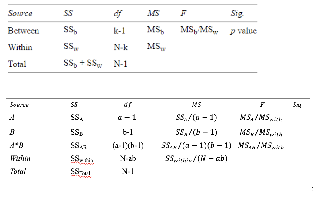
Degrees of freedom

• In ANOVA

  • dfnumerator = dfbetween

  • dfdenominator = dfwithin

• In regression

  • dfnumerator = dfregression

  • dfdenominator = dfresidual

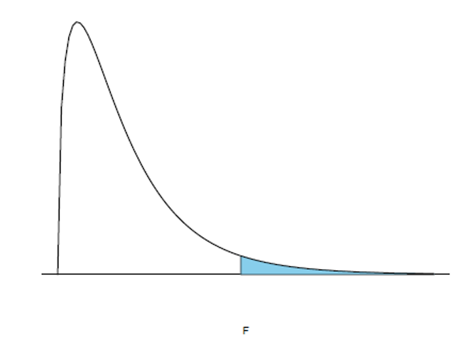
Factorial ANOVA-tests: F-distribution

In a factorial ANOVA, the null hypotheses are also tested based on an F-ratio, with the corresponding degrees of freedom

Factorial ANOVA: prediction

• Observation from group with an expected value for the response variable

• Within a group, there is random (unexplained) variation, or residual:

  • Observed response = expected response + error

• The “k-th” observation from the “i-th” group A and the “j-th” group B

  • Yijk = μ + αi + βj + αβij + εijk

    • μ = overall mean,

    • αi = group effect factor A,

    • βj = group effect factor B,

    • αβij = interaction effect A and B, and

    • εijk ~N(0,σ^2 )  indicates the error variance (unexplained)

• If there is no interaction effect between A and B, this simplifies to:

  • Yijk = μ + αi + βj + εijk

Relating Factorial ANOVA to One-way ANOVA

• Intuitively: you can also execute two separate ANOVA-tests, but:

  • .. this does not allow you to (directly) estimate the interaction effect

  • .. less power if main effect other factor is statistically significant,
       because the two factors are regarded separately

F-test for different hypotheses

• Null hypothesis 1: If H₀ holds, then σα^2 = 0 (and F=1)

  • Effect size: ηA^2 = SSA / SStotal

• Null hypothesis 2: If H₀ holds, then σβ^2 = 0 (and F=1)

  • Effect size : ηB^2 = SSB / SStotal

• Null hypothesis 3: If H₀ holds, then σαβ^2 = 0 (and F=1)

  • Effect size : ηAxB^2  = SSAxB / SStotal

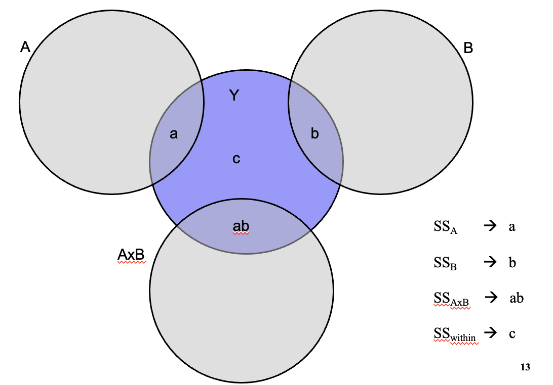
Venn-diagrams: orthogonality factor A and B

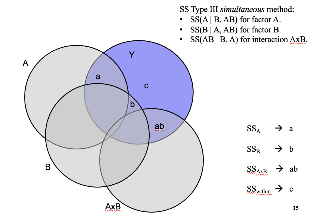
Venn-diagrams: non-orthogonality factor A and B

• SS Type III simultaneous method:

  • SS(A | B, AB) for factor A.

  • SS(B | A, AB) for factor B.

  • SS(AB | B, A) for interaction

• OR:

• SS Type I stepwise method, first A:

  • SS(A) for factor A.

  • SS(B | A) for factor B.

  • SS(AB | B, A) for interaction AxB.

• OR:

• SS Type I stepwise method first B:

  • SS(B) for factor B.

  • SS(A | B) for factor A.

  • SS(AB | B, A) for interaction AxB.

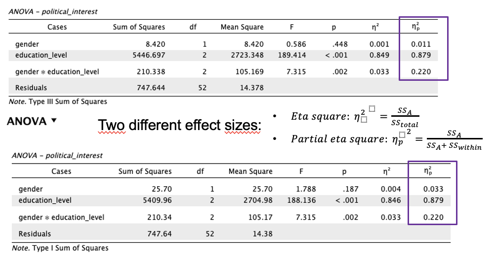
Partial Eta Squared provided by JASP

• Two different effect sizes for Type III Sum of Squares and Type I Sum of Squares

• Intuitive interpretation of Partial Eta Squared: The proportion of error that a factor (A, B, or A*B) removes by including this factor into the model after the explained variance of the other factors already has been allocated.

When group sizes are unequal (unbalanced)

• Calculate means in two ways:

  • Weighted means

  • Unweighted means

Weighted means

• Groups with more people count more

• Each cell mean is weighted by its sample size

• Reflects real-world prevalence

• The larger group has more influence

• Use when unequal group sizes are meaningful (caused by confounding between factors A & B)

Unweighted means

• All groups count equally

• Each cell mean gets the same weight

• Answers: “What would the mean be if all groups were the same size?”

• Assumes unequal sizes happened by chance

• Use when unequal group sizes are accidental

Which mean to choose?

• No uniform answer. Warner (2013) provides the following suggestions:

• Is the difference in numbers a consequence of a confounding effect between A & B? → weighted mean

• Is the difference in numbers attributable to coincidence? → unweighted mean

Factorial ANOVA: Multiple testing and Type 1 error

• When executing a factorial ANOVA, multiple (3) hypotheses are tested

• → The probability to incorrectly reject at least one of these hypotheses is larger than 5%, namely 14%:

  • 1 - (1 – 0.05 )³ = 0.141 > 0.05

• Solutions:

  • Omnibus F-test

  • Controlling family-wise Type I error rate

  • Controlling false discovery rate

  • Preregistration of hypotheses

Outliers, Laverage and Influential Points

• An outlier is a data point whose response y does not follow the (general trend of the) rest of the data.

• A data point has high leverage if it has "extreme" predictor x values.

• A data point is influential if it strongly influences any part of a (regression) analysis, such as the predicted responses, the estimated slope coefficients, or the hypothesis test results.

Causes of outliers

• Data entry errors

• Measurement erros

• Genuinely unusual values

• How to identify outliers:

  • 2 SD rule

  • Boxplot

  • Mahalanobis distance

Data entry error: Action

• Replace: if it is clear what the correct entry would hae been

• Remove: if this is not the case

Measurement error: Action

• Replace: with maximum/minimum value if the direction of the deviation is “correct”

• Remove: if entirely unclear what the “correct” value would have been

Genuinely unusual values: Action

• Depends on objective

• Keep: and if possible execute robust two-way ANOVA

• Adjust: to less extreme value and compare outcomes

• Transform: variable (e.g. log-transformation)

• Remove: and compare outcomes

Check assumption: Normal distribution of Y (outcome variable)

• Shapiro-Wilk test

  • Null hypothesis: data are normally distributed

  • If p > .05 → looks normal (OK)

  • If p < .05 → not normal (problem)

• Visually

Check assumption: Eqal variances

• Assumes all groups have the same variance/spread

• Lavene’s test

  • Null hypothesis: variances are equal

  • If p > .05 → assumption is met

  • If p < .05 → assumption is violated

• When assumption is violated/not met: Heteroscedasticity → larger Type I / Type II error due to under-/overestimating standard error (se)

• What can we do if variances are unequal?

  1. Transform the data (e.g., log transformation)

  2. Continue anyway (ANOVA is often robust)

  3. Use a robust version of ANOVA

  4. Use weighted linear regression

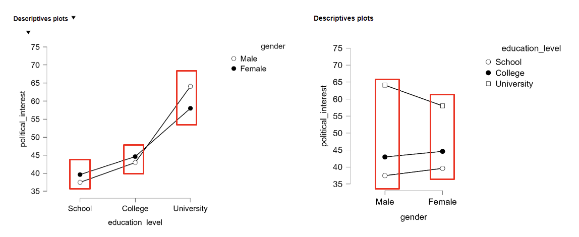
Two-WayANOVA: results

• Firstly look at the coefficient of the interaction term. Why?

  • Significant? It is not possible to clearly interpret the coefficients for the main effects.

  • Not-significant? Interpret the main effects and e.g. post-hoc pair wise comparisons.

Comparing with multiple regression

• The interaction effect can also be performed with a regression analysis:

  • Problem: 2 categorical independent variables → quantitative coding

  • Next: create interaction term → genxedu

  • Multiple regression equation: Yi = b0 + b1∗geni + b2∗edui + b3∗genxedui + εi

• Is undesirable method here due to type of independent variable ”level of education” (qualitative)!

  • Regression assumes that independent variable is dichotomous or has interval/ratio scale

Extra: estimating “simple” effects

• If there is a statistically significant interaction, you can decide to estimate simple effects: ”the effect of factor A per level of factor B” and “the effect of factor B per level of factor A”

• Alternative: estimating simple effects via separate one-way ANOVAs. Disadvantage is lower power.

• In JASP, these simple effects can be estimated directly (with Bonferroni-correction for multiple tests)