Module 10 - Correlation and regression

Correlation test

Goal is to evaluate if there is an association between two numerical variables (whether one variable trends up/down as the other changes)

Key notes about correlation tests

1. No implied causation

2. Both variables are assumed to have variation

3. Not used for prediction, only to evaluate association

Correlation strength

Measured by Pearson’s correlation coefficient (r), the population parameter is given the Greek letter ⍴ (rho). Can take any value from ⍴=-1 to ⍴=1. ⍴=-1 indicates a perfect negative correlation. ⍴=0 indicates no association. ⍴=1 indicates perfect positive correlation

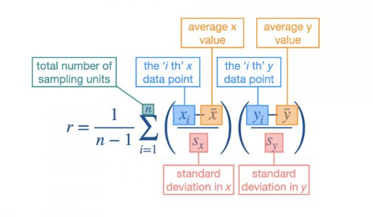
The expression for calculating the correlation coefficient from a sample. Covariation (how much one goes up when the other changes) is found within the brackets, then sum over all sampling units and divide by degrees of freedom (take the average covariation among sampling units)

Assumptions behind a correlation test

1. Each pair of numerical values is measured on the same ampling unit

2. Numerical values come from continuous numerical distributions with non-zero variation

3. If there is an association between the variables, it is a straight line

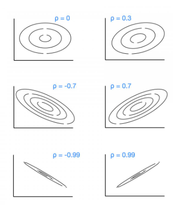
Bivariate normal distribution

An extension of the normal distribution for two numerical variables that allows for an association between them. Shows contour lines that represent variation. The tighter the lines are, the closer to perfect correlation

Null and alternative hypotheses for the correlation test

Null hypothesis: correlation coefficient is zero ⍴=0, OR can be directional, ⍴≤0 (or ⍴≥0)

Alternative hypothesis: correlation coefficient is not zero ⍴≠0, OR directional, ⍴>0 (or ⍴<0)

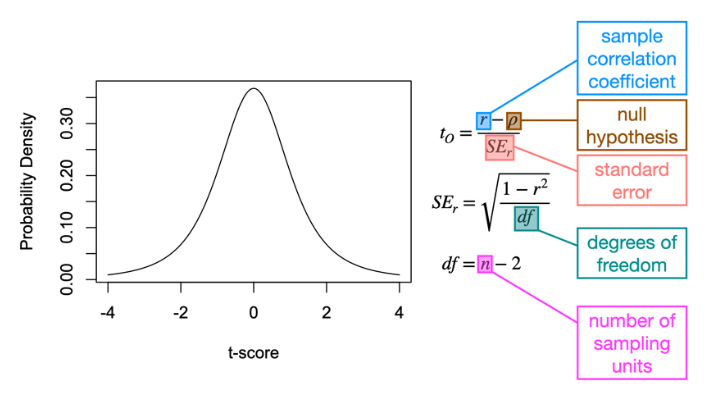
Null distribution for a correlation coefficient

T-distribution. Correlation tests are a special case of a single-sample t-test. Use the same machinery as a single-sample t-test. Reject the null hypothesis if t_O>t_C or p<⍺. Fail to reject if t_O≤t_C or p≥⍺

Scientific conclusions for a correlation test

Non directional:

• Reject the null hypothesis and conclude that there is evidence of an association between the two numerical variables.

• Fail to reject the null hypothesis and conclude that there is no evidence of an association between the two numerical variables.

Directional:

• Reject the null hypothesis and conclude that there is evidence of a positive (or negative) association between the two numerical variables.

• Fail to reject the null hypothesis and conclude that there is no evidence of a positive (or negative) association between the two numerical variables.

Linear regression test

Is the statistical test used to evaluate whether changes in one numerical variable can predict changes in a second numerical variable

Key points about linear regression tests

• focus is on prediction (one variable is predictor variable, other is response variable)

• sampling error occurs only in the response variable

• in experimental studies: reflects a causal relationship, predictor variable/independent variable is manipulated, response/dependent variable is measured

• in observational studies: predictor and response variables depend on the research question — want to make predictions about the response variable

Linear equation

y_i= a + bx_i

Shows that the response variable is equal to the intercept parameter plus the slope parameter * the predictor variable

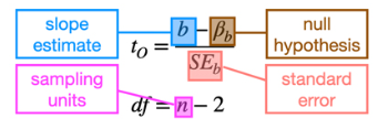
Slope (b)

Describes the relationship between numerical variables. It is the amount that the response variable increases or decreases for every unit change in the predictor variable. Positive values describe an increasing relationship, zero value indicates no relationship, negative describes a decreasing relationship

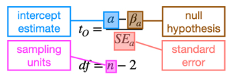
Intercept (a)

The value of the response variable when the predictor variable (x) is at zero. Changing the intercept raises/lowers the line, but does not change the relationship between the variables

Three components to the statistical model

Systematic component, random component, link function

Systematic component

Describes the mathematical function used for predictions. For linear regression is the linear equation. Parameters are the intercept (a) and slope (b)

Random component

Describes the probability distribution for sampling error, as well as where it emerges in the model. For linear regression, is the normal distribution for the response variable. Illustrated as “coming out the screen towards you” for each data point. The mean value can change across x, but the standard deviation does not change

Link function

Connects the systematic component to the random component. States that the mean of the normal distribution is the same as the predicted value from the linear equation

Fitting the statistical model

Estimation of the intercept and slope that best explains the data — done by minimizing residual variance

Residual variance — sum of squares

The average squared residual value across all data points — the difference between the observed data point and the predicted value

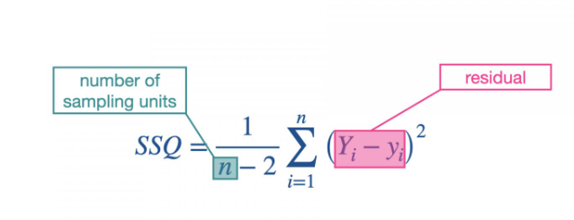
Calculation for sum of squares

1. Calculate the residual for each data point

2. take the square of each residual

3. Sum the squared residuals across all data points

4. Divide the degrees of freedom, which are df=n-2

Minimizing the sum of squares

The process for fitting the statistical model to data — varying the slope and intercept parameters until you find values that minimize the residual variance

Hypothesis testing for linear regression

Done on the parameters of the systematic component. Test hypotheses for the intercept and slope.

Intercept null and alternative hypotheses

Null: Intercept is not different from a reference value, or a=βa in symbols, H_O: a≤β_a

Alternative: Intercept is different from a reference value, or a≠βa in symbols, H_A: a>β_a

Slope null and alternative hypotheses

More common than for an intercept — usually whether it is different from zero.

Null: Slope is not different from a reference value, or b=βb in symbols, H_O: b≤β_b

Alternative: Slope is different from a reference value, or b≠βb in symbols, H_A: b>β_b

Linear regression test

Works by locating critical t-score and comparing to observed t-score. Statistical decision is:

• Reject the null hypothesis if the observed score is greater than the critical score (i.e., t_O>t_C) or if the p-value is smaller than the Type I error rate (i.e., p<⍺).

• Fail to reject the null hypothesis if the observed score is less than or equal to the critical score (i.e., t_O≤t_C) or if the p-value is larger or equal to the Type I error rate (i.e., p≥⍺).

Scientific conclusions for a linear regression test

Depends on parameter under consideration. Could be non-directional or directional. Below are non-directional:

Intercept:

• Reject the null hypothesis and conclude there is evidence that the predicted response variable is different from the reference (β_a) at x=0.

• Fail to reject the null hypothesis and conclude there is no evidence that the predicted response variable is different from the reference (β_a) at x=0.

Slope:

• reject the null, there is evidence that changes in the predictor variable can be used to predict changes in the response variable

• fail to reject the null, there is evidence that changes in the predictor variable can predict changes in the response variable

Four main assumptions for a linear regression

1. Linearity

2. Independence

3. Normality

4. Homoscedasticity

Linearity

Response variable can be described as a linear combination of the predictor variable. Assume the systematic component is y= a+bx, means relationship is assumed to be a straight line. Evaluated qualitatively

Assumptions of linearity met

The data shows a straight line relationship between the predictor variable and the residuals. If the relationship is described by a straight line, then the residuals will not have a trend

Assumptions of linearity violated

The residuals may have a trend to them, may often look like a smiling or frowning face (curved relationship to them)

Independence

Assumption that residuals are independent of each other across the predictor variable. Violations may occur when there is repeated sampling of the same sample units or there is a spatial/temporal relationship among sampling units. Can guard against it be ensuring units are selected at random. Evaluated qualitatively

Assumptions of independence met

Look at the pattern among adjacent residuals, there is a switch between positive and negative residuals.

Assumptions of independence violated

Residuals are not independent, may have runs of positive and then negative

Normality

Assumption that residuals are normally distributed (not the data itself). Evaluated qualitatively by looking at a histogram of the residuals as densities with a normal distribution overlaid on top with a mean of zero and a standard deviation matching that of the residuals. Can also be evaluated quantitatively with a Shapiro-Wilks test

Assumptions of normality met

The histogram of residuals will look similar to the reference normal distribution. Residuals are normally distributed.

Assumptions of normality violated

Statistical population may have a skewed or unusual distribution. May also violate assumptions of linearity. residuals are not normally distributed, may have more density in the middle and less in the tails than expected for a normal distribution, or may be skinnier.

Shapiro-Wilks test

Statistical test used to quantitatively evaluate the assumption that the residuals are normally distributed.

H_O: The residuals are normally distributed, H_A: The residuals are not normally distributed

If p≥α then we fail to reject the null hypothesis, no evidence to suggest that the residuals are not normally distributed

Homoscedasticity

Assumption that the residuals have the same variance across the predictor variable. Can be evaluated qualitatively by looking at a plot of residuals against the predictor variable

Heteroscedasticity

If the residuals have little variation along some parts of the predictor variable and large amounts at others. Can be caused if residuals are not well described by a normal variation.

Assumption of homoscedasticity met

Straight line relationship between predictor variable and residuals. There is roughly equal variance across the predictor variable (on positive and negative sides of the predictor variable).

Assumptions of homoscedasticity violated

Residuals have small variance at low values of the predictor variable and increased variance at high values, for example.

If assumptions are violated

No simple 1:1 map between violations of assumptions and trustworthiness of statistical results. Sometimes violation has little impact on robustness of the statistical conclusions, sometimes minor violations can alter the statistical conclusions.