S101 Derivations, definitions, and formulae

Reasons to estimate consumer demand systems

1. Welfare analysis (from price changes)

2. Cost of living indices

3. See how consumers substitute goods in response to price changes (also linked to welfare analysis)

Demand system

A system of equations linking price and quantity demanded of goods that must be derived as the solution of a consumer problem for a given utility function.

I.e. demand systems must be invertible - not every equation system that links quantities and prices is a demand system.

CES utility - finding EQ demand

CES utility:

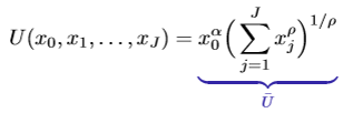
Take FOCs for x0 and xj to obtain expressions for marginal utilities

Then divide the FOC wrt good j by the FOC wrt good 1 to obtain an expression for xj in terms of prices and good 1, then replace this in the BC.

Solve for x1 in terms of x0, then solve for x0 in terms of parameters and income.

Axioms for Economic Rationality

1. Reflexivity - any bundle is always weakly preferred to itself (trivial but required)

2. Completeness - any two bundles of goods can be compared (no bundles are outside the preference ordering)

3. Transitivity - if a is preferred to b and b is preferred to c, c cannot be preferred to a

4. Continuity - If x⪰y , then there exists a bundle z close to x such that z⪰y; and similarly if y⪰x

5. Non-satiation (monotonicity) - more of any good is always preferred to less

Weak axiom of revealed preferences (WARP)

If A and B are feasible and a person chooses A, a change in prices that causes A and B to still be feasible should not cause B to be chosen over A.

Properties of demand that follow from the budget constraint

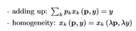
Adding up: BC always binds due to non-satiation

Homogeneity: no money illusion - if income and prices rise by the same proportion, consumption won’t change

Engel Curves

Show how demand changes has income changes, generated by fixing prices and looking at demand as a function of income.

Key point is that different goods have different slopes, so income elasticities cannot be constant for all goods

Dual approach for obtaining demand systems (i.e. expenditure minimisation problem)

Different to ‘primal approach’ utility maximisation problem used to create a Marshallian demand system

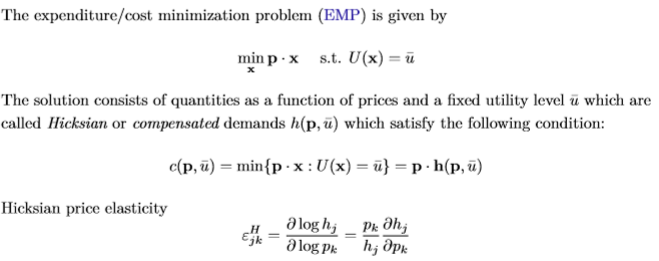
Duality of this approach is shown through the fact that the indirect utility (utility resulting from UMP for Marshallian demand) is the same as the fixed utility level for the EMP only if the resulting cost function (costs resulting from solving the EMP for Hicksian demand) is equal to income.

You can use this to your advantage (e.g. when you have already derived Marshallian demand, you can obtain indirect utility wrt y and then sub in y = c(p,u*) and rearrange to get the cost function (and then differentiate that to get Hicksian demand via Shephard’s lemma

Properties of cost functions

1. Homogeneous of degree 1 in prices

2. Continuous in prices and utility

3. Non-decreasing in prices, strictly increasing in utility for positive prices

4. Concavity in prices (ensures negative definiteness of the SOC)

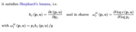
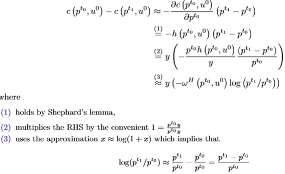
5. Satisfies Shephard’s lemma:

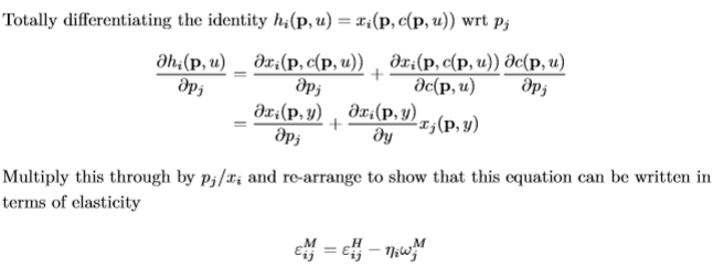
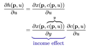
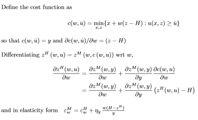
Deriving the Slutsky equation

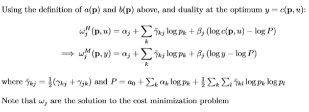
Almost Ideal Demand System (AIDS): process for estimation

1. Take derivative of log cost function wrt. log p to get an expression for the income share of each good (Shephard’s lemma)

2. Use duality at the optimum (cost function = income) to sub in y where possible

3. Final system should have the following form:

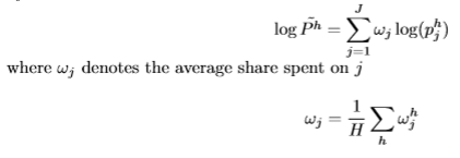
4. Approximate P with the Stone Index

5. Add an i.i.d. error to each household’s equation in the system, and estimate parameters using simple regression on a micro dataset (prices, incomes, demand levels)

General formula for a cost of living index

Every utility function will give a different CoLI, since you need to decide the initial representative basket of goods

CoLI with Cobb-Douglas preferences

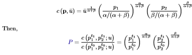
Solve for Marshallian demands to get indirect utility then solve for the cost function

Key points:

1. Independence of base - P does not depend on utility levels

2. Normalising parameters to alpha + beta = 1, setting prices in the base year equal to 1, and then taking logs of P gives the following:

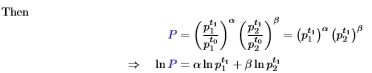
Ln(P) is a geometric mean weighted by budget shares, i.e. it is the Stone Price Index.

P measures the CoL assuming that the effect of a price change depends on the share consumers spent on goods 1 and 2 (not the actual amounts they spend)

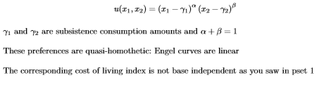
CoLI with Stone - Geary preferences

Why isn’t comparing indirect utility a useful measure of welfare costs from a price change

Any monotonic transformation of the utility function will yield different indirect utilities, and hence a different welfare cost (despite giving the same optimal consumption bundle)

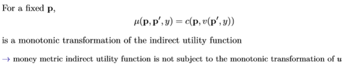
Money metric indirect utility functions

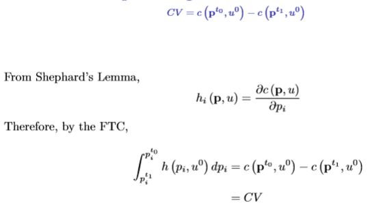
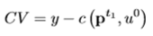
Compensating Variation as a £ measure of welfare costs

Amount of money needed to compensate an individual for a change in prices so that their utility remains the same as it was before.

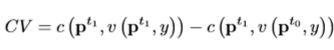
First term is equal to income (cost function at t = 1 prices and t = 1 utility) due to duality

Additionally:

Amount of money needed to compensate an individual for a change in prices so that their utility remains the same as it was before. First term is equal to income (cost function at t = 1 prices and t = 1 utility) due to duality:

Additionally:

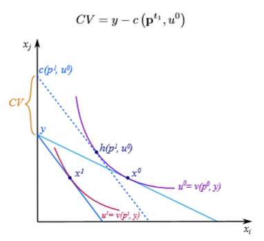
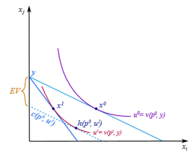
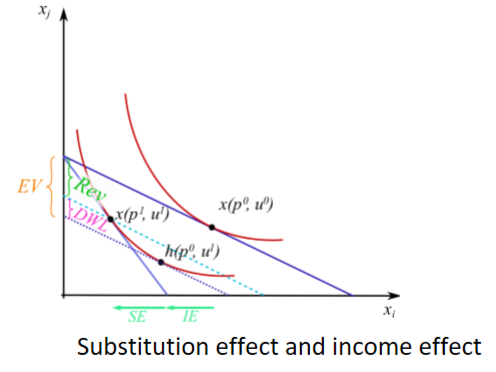
Compensating variation graphs (demand curves and indifference curves)

Equivalent variation

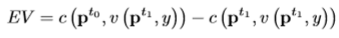
How much money would I need to give away such that I would have today’s utility at yesterday’s prices.

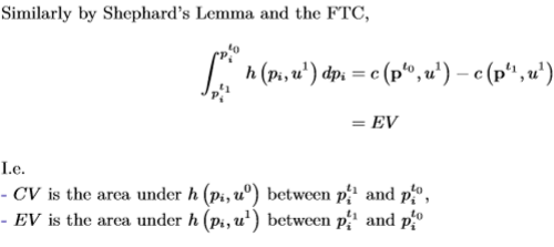
In this case, income is the second term - so EV is the difference between the cost of today’s utility at yesterday’s prices and today’s income:

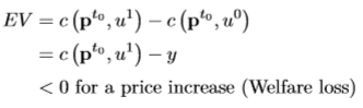
Equivalent Variation diagrams

Comparison between EV and CV

Higher utility shifts the Hicksian demand curve to the right if normal, and to the left if inferior (always holds since the cost function is strictly increasing in the level of utility)

The difference between EV and CV is driven by income effects. When the price of a normal good rises, demand falls due in part to the income effect, but the consumer is more sensitive to income at lower utility levels, hence the CV (which starts at the higher indifference curve of prices at 0, utility at 0) will have stronger effects than EV. For a utility function without income effects (i.e. quasi-linear preferences) EV = CV.

EV and CV size comparison for normal and inferior goods

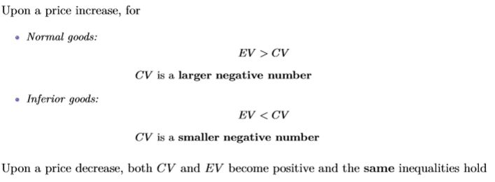
EV and CV are different because of income effects, and the different marginal utilities of income. For CV, the utility level you are trying to compensate for is higher (i.e. original utility with original prices), so since the utility of income is diminishing marginally, it requires more income to compensate. For EV, the utility level is lower (new utility with higher prices), so the the amount of income required to take away to achieve that utility level at old prices is lower.

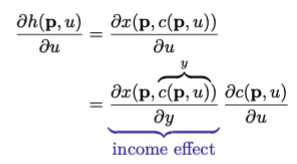
The key point is that dc(p,u) / du is always positive, but is smaller for EV than it is for CV due to the differences in marginal utility of income.

Consumer surplus

Area under the Marshallian demand curve:

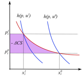
With no income effects, CV = EV = change in CS

With income effects, change in CS lies between EV and CV

It is the most common welfare measure, and is an intermediate measure between CV and EV, but doesn’t have an immediate interpretation in terms of utility theory

Laspeyres price index

Under Leontief utility (perfect complements - the representative basket is always consumed in the same ratio

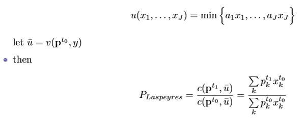
This is an ideal index - chooses some level of utility and asks how much more expensive is it to achieve that utility when the prices change

Paasche price index

Key difference between Paasche and Laspeyres: Paasche uses utility at t = 1 as the base (‘ideal’) utility, whereas Layspeyres uses utility at t = 0

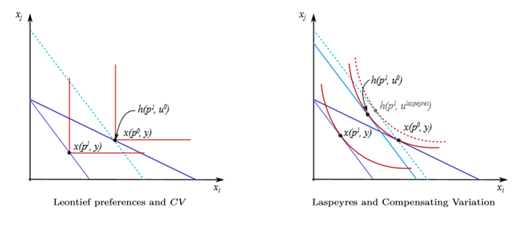
Over and underestimation results for Laspeyres and Paasche when preferences are not restricted to being Leontief

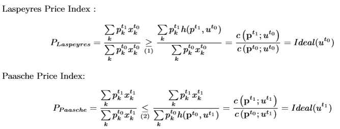
Laspeyres overestimates compensating variation

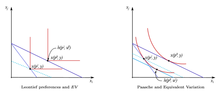
Paasche underestimates equivalent variation

Laspyeres and CV: Diagram

Paasche and EV: Diagram

Estimating CV: First order Taylor approximation

CV can thus be estimated using data on income, consumption shares and prices

Estimating CV: Second order Taylor approximation

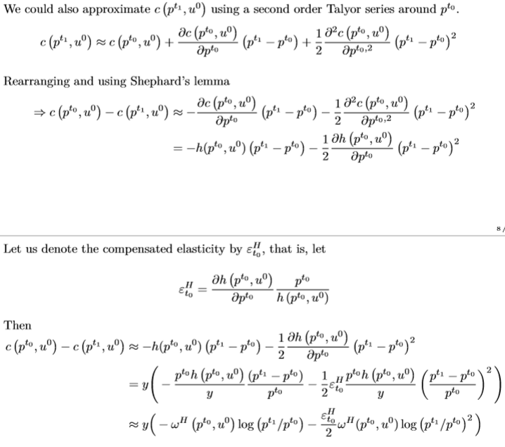
The elasticity term captures substitution effects, but now requires that there be price variation in the data when estimating CV

Banks, Blundell and Lewbel (1996) argue that it is empirically necessary to estimate price elasticities to properly evaluate welfare effects of large price changes, but when prices are small, first order approximations perform adequately.

Estimating CV: AIDS

Estimate the almost ideal demand system as gone over in other cards, then back out cost functions to estimate CV. Would need data on income, shares, and prices to estimate the CV, and could not use aggregate data.

2nd Welfare Theorem + why it fails

Any Pareto efficient outcome can be reached by redistribution of endowments and then letting the market run its course

Fails because redistribution of endowments (basically ‘abilities’ is not feasible so the gov’t must use distortionary taxes and transfers, incurring an equity / efficiency tradeoff.

Lump-sum taxation and deadweight loss

Taxes where the burden can’t be reduced by changing consumer behaviour. They are idealised as they imply that taxes only vary with endowment (i.e. ability)

Deadweight loss arises due to the behavioural response to a tax. it is the additional welfare loss of a tax above the revenue it creates. The magnitude of the inefficiency is determined by the extent to which consumers change their behaviour to avoid the tax.

DWL: Diagram (on indifference curves, easily recognisable on supply+demand curves

Derivation of Harberger’s Formula

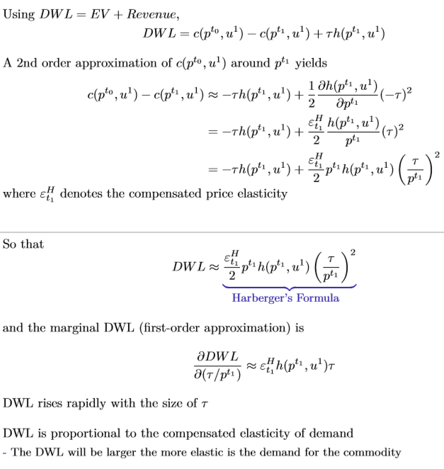
Deadweight loss formula

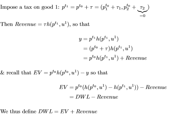
Remember, income effects of taxation are non-distortionary (i.e. consistent with second WT). Taxes only become distortionary due to the behavioural response

Tax incidence

Statutory incidence of a tax: doesn’t describe who bears the tax, so does not = economic incidence. Taxes can be shifted since they directly affect prices which affects quantities, which then affects other prices.

Tax incidence is borne by those who cannot easily change their behaviour. Therefore:

Static labour supply model: consumer’s problem

Interior solutions will take the form of:

so the wage rate is the rate at which the consumer is willing to give up leisure in return for additional consumption

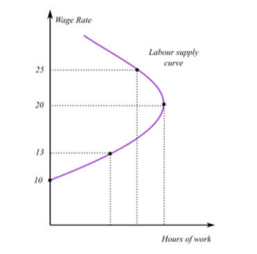
Decomposed total effect of a change in w (i.e. the price of leisure)

Income effect: as income increases, workers tend to supply less labour to ‘spend’ the higher income on leisure

Substitution effect: as income rises, the opportunity cost of leisure increases and workers supply more labour

Overall effect depends on which effect dominates, and this may vary for different wage rates (if sub effect is stronger, labour supply curve is upward sloping, opposite true for if the income effect is stronger)

Extensive margin in static labour supply model

Static labour supply: formal derivation of slutsky equation

Blundell, Duncan and Meghir as a key application for labour supply models (basic idea)

Motivation was to estimate the DWL of taxation on married or cohabiting women with employed partners (the most likely group to change their labour supply due to a change in economic conditions)

Exploits 1980s UK tax reform. Affected different earnings groups at different times, so you can use difference in difference

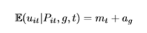
Specification of the error term for TWFE method (additive for common trends) allows for taste heterogeneity as long as the differences across groups remain fixed over time, as well as common time shocks.

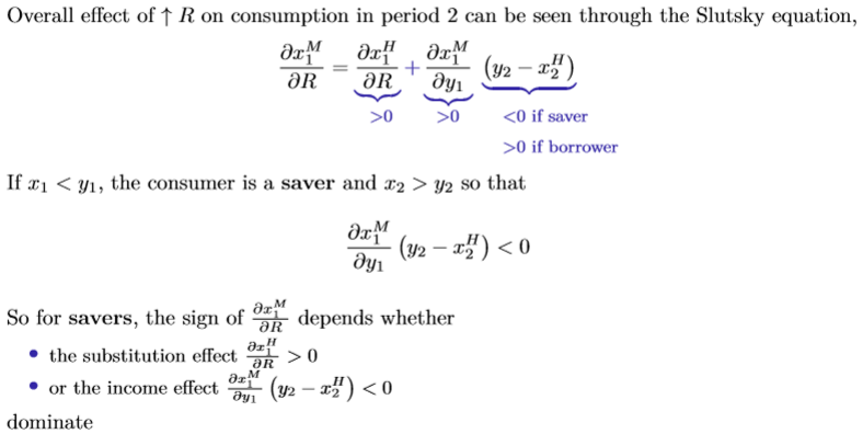
Derivation of Slutsky equation for intertemporal choice model

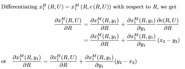
Where R = 1/(1+r)

Pareto conditions (i.e. for an allocation to be Pareto efficient)

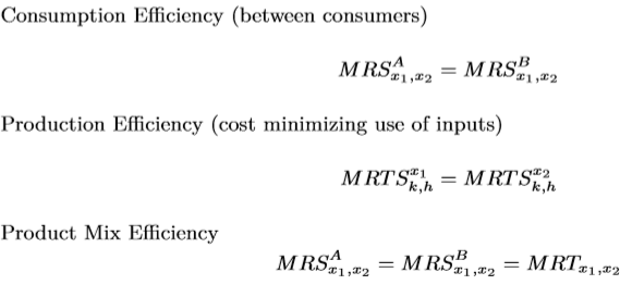
MRT is the marginal rate of transformation - equal to the slope of the PPF

Basic policy guidance under general theory of second best

1. With interdependencies between markets, policy should be guided by the principle that distortions can offset each other and that new distortions can counteract existing ones rather than restoring Pareto conditions in some markets

2. With no interdependencies between markets, policy should be guided by the principle that Pareto conditions should be satisfied in independent markets (if possible)

James Meade Tariffs (two interdependent markets, one with a removable tariff, one with an irremovable tariff)

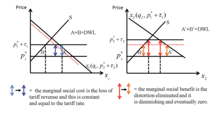
Reducing the tariff in market 2 has two effects

Reduction of distortion (DWL) in market 2, which is diminishing marginally the more the tax is removed

Reduction of demand in market 1, so there is lost tariff revenue (constant marginally and equal to the tariff rate)

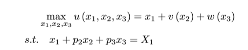
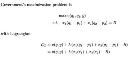
Ramsey pricing: Government’s problem (max consumer utility subject to their budget constraint)

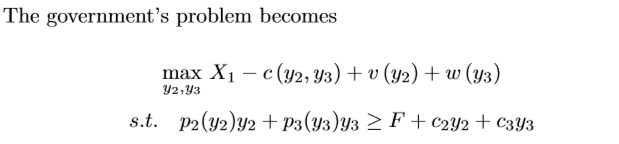
Find FOCs and sub in consumer’s FOCs from their maximisation problem:

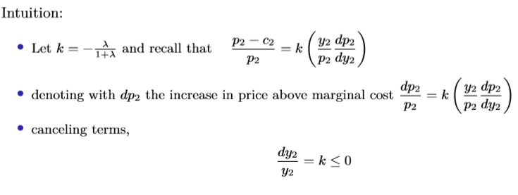
Ramsey pricing: key result (independent markets)

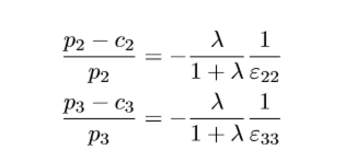
Goods that are elastic in demand should be priced close to marginal cost

Goods that are inelastic in demand should be priced further above marginal cost

It is optimal to price both the public goods above MC (with interdependent markets, it is not optimal to try to set price equal to MC for a good either)

Ramsey rule is a prescription of how to restrict output - the quantity of each good should be reduced proportionately, and by the same percentage

See notes for modified rule with interdependent markets

Diamond and Mirrlees production efficiency: assumptions

1. Competitive markets: prices taken as given for consumers and producers

2. Constant returns to scale technology in production of all commodities

3. Full flexibility in choosing taxes on all commodities and factors of production in the form of wedges

4. Revenue requirement for the gov’t is R

5. No lump-sum taxes

6. Individualistic social welfare function

7. Non-satiation for at least one good

Diamond and Mirrlees production efficiency: key result

If all of the assumptions hold, the second best optimal tax system maintains the economy on the PPF. This is because with 0 profits, welfare is only determined by consumer prices (and how choices are influenced by them. Hence, any utility level attained with production inefficiency can be attained when the inefficiency is removed, so production inefficiencies only add distortions without correcting others or generating benefits.

So to meet the revenue requirement, distort the consumption side (assumed to be independent of production side) and maintain productive efficiency (doesn’t necessarily mean that you don’t tax producers at all, just means that taxes shouldn’t stop them producing on the PPF)

Basic production efficiency example: diagram

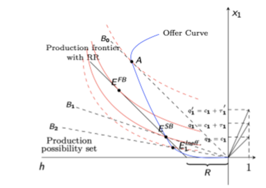
On the ideal (no tax) budget line (q1 = c1) the consumer’s preferred bundle would be A, but that is unattainable (reminder that c1 is equal to the producer’s price due to perfect competition - q1 is the price that the consumer sees)

If we allow for lump sum (non-distortionary) taxation, the consumer’s budget constraint shifts by exactly the same amount as the PPF for the revenue requirement. This gives E(fb) which satisfies all Pareto conditions but is unattainable since only distortionary taxation is possible

Therefore, the government sets the consumption tax at t1, changing the consumer’s BC to B1, which meets the relevant indifference curve at E(sb). This point is on the PPF, maximise consumer utiltiy, but doesn’t meet the Pareto condition of MRS = MRT so is not first best

Setting the tax too high to t’1 woudl result in BC of B2, and a consumer maximisation point of E(ineff) which is below the PPF.

Application of production efficiency result: input taxes

If you tax inputs differently depending on the sector, then the MRTS is not going to be the same between industries, and the economy will not be production efficient. You can reallocate inputs to increase production of both goods.

Ramsey taxation: government’s problem and FOCs

Note we have added the exogenous income term y = 0 to the consumer’s BC so that we can define the indirect utility of consumers

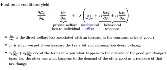
Ramsey taxation - steps breakdown to reaching optimal formula

1. Sub in Roy’s identity to the FOC

2. Define Marshallian demand as a function of exogenous income y = 0 to yield a Slutsky eqn that you can sub into the FOC

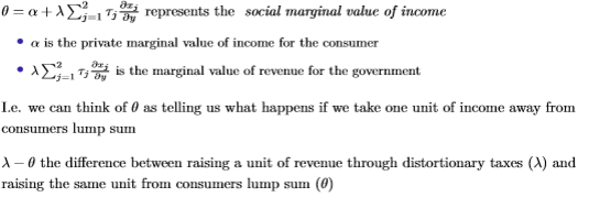
3. Rearrange and define theta as social marginal value of income term

4. Rearrange to get the following result

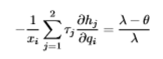
5. Final step to get optimal tax formula:

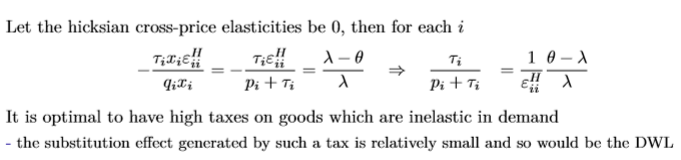
Generalises easily to the many goods case, since Hicksian cross-price elasticities are 0

Roy’s identity

Where remember that q(i) is the price that is faced by the consumer, not the quantity, and v is the consumer’s indirect utility of consumption.

Alternatively written as below:

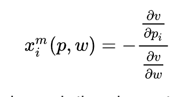
w = y in this case.

Social marginal value of income - key facts

Ramsey taxation with two equity considerations (i.e. two types of consumer): key result and interpretation

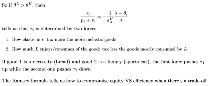
The general formula is given below - useful because often elasticities in questions are different between types. Most often, though, we will assume that cross elasticities are 0.

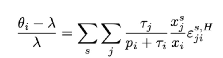
Key terms that are defined in the Ramsey taxation model with equity considerations

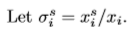
where superscript s denotes the consumer’s type (L or H)

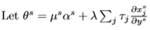
Similar to the social marginal value of income before, but this time the private marginal value of income for consumer of type s is weighted by the relevant government weighting.

Can be interpreted as the social marginal value of income for consumer s, considering both the direct welfare effect on the consumer and the indirect effect through changes in government revenue, weighted by the goverment’’s valuation of the welfare of consumer s.

Weighted average of the social marginal values of income across all consumers, with the weights being the shares of consumption of good i.

Reflects how changes in income, mediated through consumption, affect social welfare.

Lambda is the marginal cost of public funds, so lambda - theta = the difference between raising a unit of revenue via distortionary vs lump sum taxes

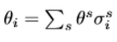
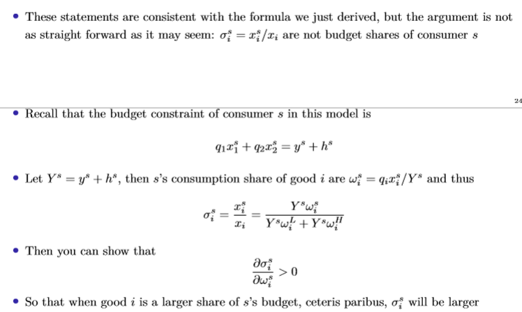
Reason that goods that constitute a large share of the budget of the poor should, ceteris paribus, be taxed at a lower rate

Does the Mirrlees model allow for commodity taxation?

Yes

Mirrlees: single crossing property

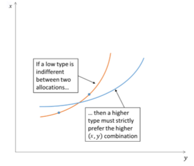
Implies that high skilled will never earn less income than the low skilled

Tangency points between the gov’t’s chosen consumption function and the indifference curve of the low skilled cannot be tangency points for the high skilled. High skilled indifference curves are flatter.

Intuitively, single crossing ensures no envy, which allows the gov’t to handle incentive compatibility constraints.

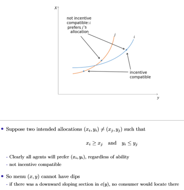
Mirrlees: incentive compatibility restriction

Agents cannot prefer another agent’s bundle to their own, in order to incentivise them to truthfully report their income

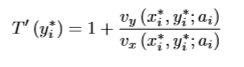
Mirrleesian tax problem

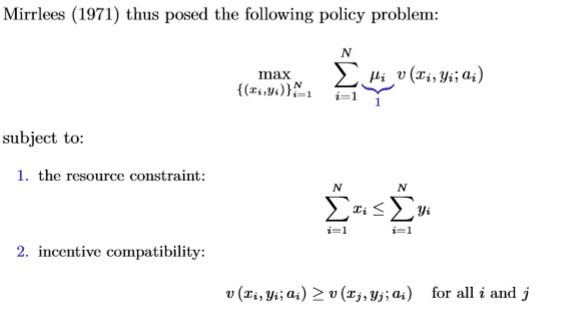
Government’s tax design is equivalent to specifying a menu of (x,y) such that i chooses (x(i), y(i)) associated to her optimal marginal tax rate.

Mirrlees: individual’s problem

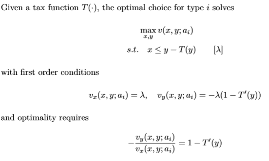
Therefore the optimal MTR for individual i is as below:

Mirrlees: diagram

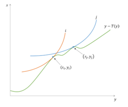
Government chooses green line as a consumption function c(y) that must be incentive compatible and satisfy the resource requirement

Mirrlees: Key result

Mirrlees: Intuition that the marginal tax rate cannot be 100% or higher

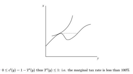
Downward slopes in the consumption function are not incentive compatible

Mirrlees: Intuition that MTR must be at least 0 (ruling out an earned income tax credit) (simple two agent case)

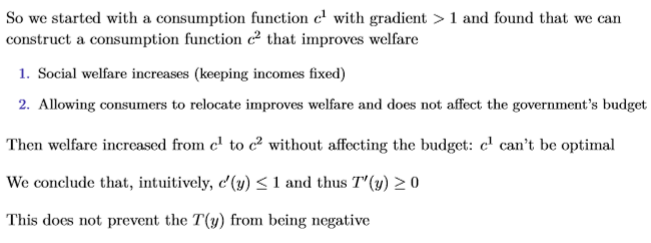
c² is designed such that, keeping income fixed, the increase in consumption for L is exactly matched by the decrease in H, so aggregate income and consumption stay the same. Since marginal utilities are higher for type L, welfare increases as a result of following this consumption function.

Letting consumers relocate to utilmax positions on c² still does not affect the gov’t’s BC.

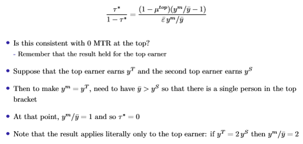
Mirrlees: Intuition that MTR on the top earner must be 0 (simple two agent case)

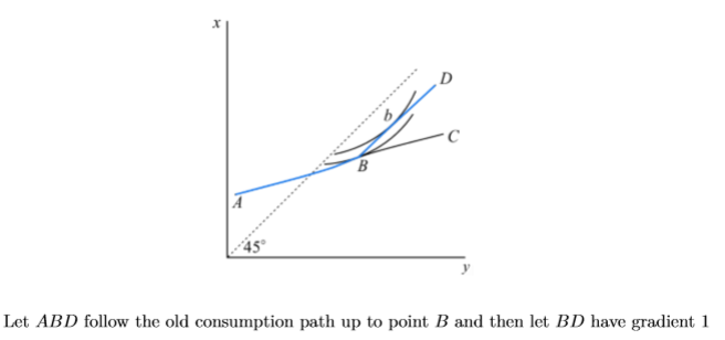
The top consumer now will locate at b so she is better off.

Reducing the MTR to 0 for the top earner is less distortionary, so she works more and earns more income / consumption. If you kept it above 0, top earner would not work those extra hours. Therefore, the tax revenue is unchanged and the top earner is better off, so it is a Pareto improvement to have a consumption function with slope 1 (0 MTR) on the top earner.

Importantly, this assumes that you can identify your top earner ex ante, and adjust taxes around her. Thus there is limited policy relevance.

Revenue maximising income tax: Laffer curve example

Key point is that this elasticity wrt taxable income can be estimated

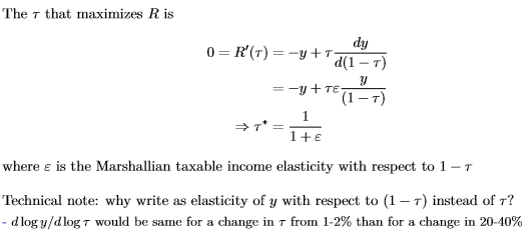
Saez optimal top bracket tax rate

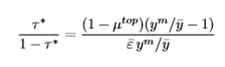
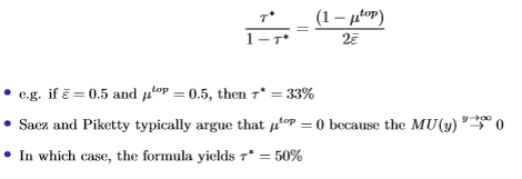
Decreases in welfare weight of top bracket earners

Decreases with elasticity of taxable income (efficiency result)

Increases with y^m / y(bar) (note this is endogenous to the tax rate, but can be seen to be roughly constant for incomes above $200K to close to the very top).

With y^m / y(bar) equal to 2, and Diamond derives the following result with Pareto skill distribution:

Optimal top income tax rate with a zero top rate (bounded distribution)

Saez optimal top income tax rate calculation: key steps

1. Identify dW = dM + dB (balances the need for revenue against distortions)

2. Work out out mechanical effect dM (changes in revenue)

3. Work out behavioural response dB (no income effects, substitution only) and rewrite using elasticity of taxable income

4. Equalise dM and dB to the welfare effect dW, which is calculated as the social marginal value of consumption for top bracket taxpayers multiplied by the mechanical effect dM (this is the direct welfare loss from raising additional revenue from top earners, given the gov’t’s valuation of their consumption)

5. Rearrange expression and divide by y(bar)

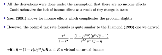
Saez optimal top income tax rate - adding income effects

Key points to remember when deriving elasticities

(Using income elasticity as reference, but true for all) don’t just differentiate x wrt. y - don’t forget to multiply by y/x as well

When deriving price elasticities, you have to remember to derive both own price and cross price elasticities unless specifically told to derive only one of them.

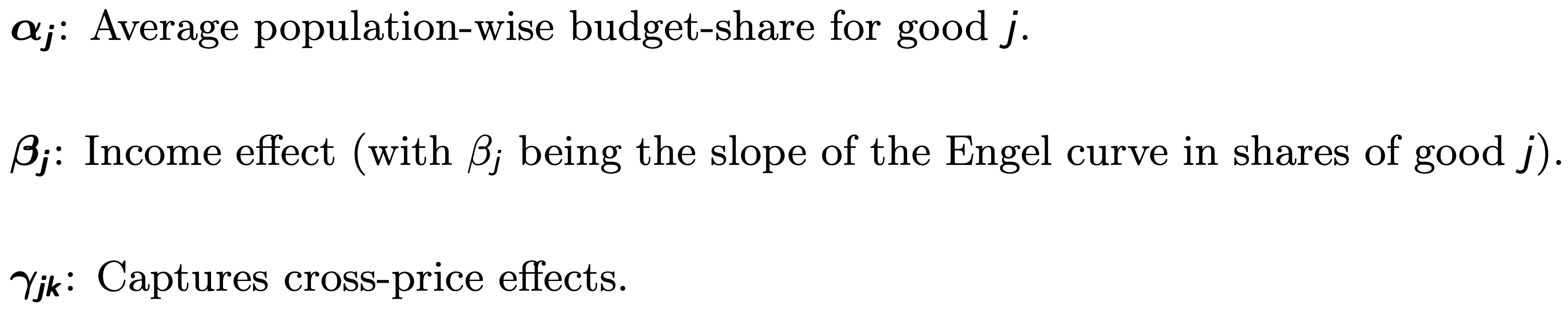
AIDS: coefficient meanings

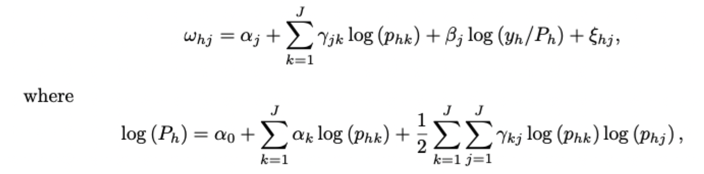
Recall AIDS as above:

Stone price index

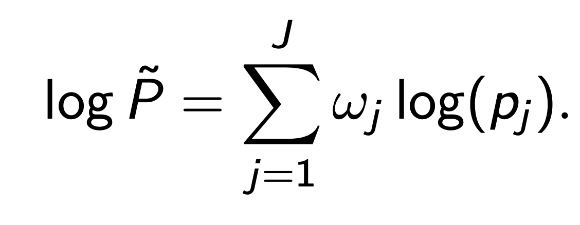
The log price level is the weighted average of all log prices by budget shares.

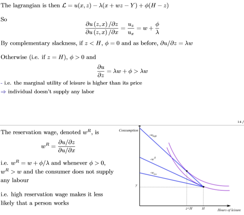
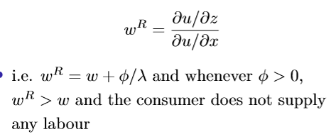
Optimal reservation wage in static labour supply model

Complementary slackness fails, so new constraint is added to the Lagrangian: z = H.

Therefore, the reservation wage at which this constraint is met is define as below:

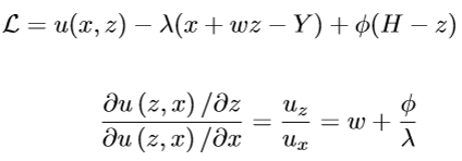
Non-participation occurs when the wage offered is less than the reservation wage. In this case, there is no ambiguity - higher wages will always make individuals more likely to enter the job market and start working.

What is added onto the wage in this case is the ratio between the marginal disutility of the first few units of labour and the marginal utility of income. Remember that this is a CORNER SOLUTION: therefore leisure has a discontinuity in wages, can’t interpret this as the result of a continuous change in parameters.

Blundell, Duncan and Meghir as a key application for labour supply models (extensions)

1. control for participation using selection correction. adding the inverse Mills ratio as a regressor to the error term estimate, (derived using a participation equation)

2. Introduce non-labour income (i.e. the difference between the value of consumption and total labour income)

3. Discontinuity in the tax schedule: they condition out observations close to the kink and add a selection term

Blundell, Duncan and Meghir (results)

All income effects are negative, consistent with the theory, with the strongest effect for mothers with 3-4 children.

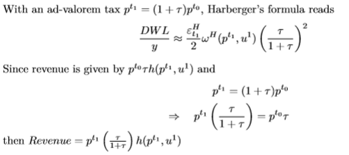
DWL for different income groups can can also be estimated using Harberger’s formula.

Harberger’s formula with an ad-valorem tax

Problems with consistently estimating a cross sectional model of labour supply

1. Net of tax, w is endogenous to the choice of hours (simultaneous causality) giving a downward bias in estimated wage elasticity

2. If individual preferences are convex then there should be bunching at convex kinks which are caused by differing marginal rates of taxation in modern progressive systems

Does the deadweight loss of a tax depend on whether the labour supply rises or falls in response to a tax increase?

Not directly. The DWL depends on the behavioural response to the tax rather than necessarily whether labour supply rises or falls as a result of this. What matters is the substitution effects relative to the income effects.