decision trees

decision tree

= method for learning discrete valued target functions in which the function to be learned = represented by a decision tree

Goal= build d.t. to classify examples as +ve or -ve instances of a concepts using supervises learning from a training set

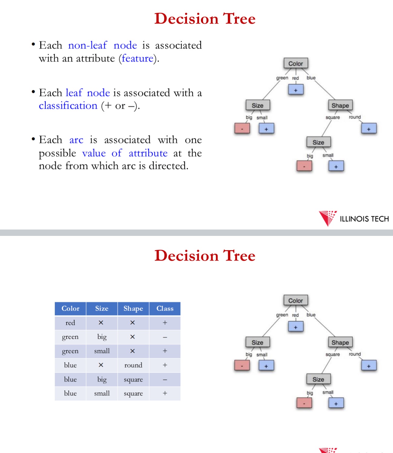
d.t. is a tree where:

• each non-leaf node = associated with an attribute (feature)

• each leaf node has associated with it a classification (= or -) i.e. +ve and -ve data points

• each arc = associated w 1 possible value of the attribute at the node from which the arc is directed

Generalisation is allowed I.e. more than 2 classes can exist

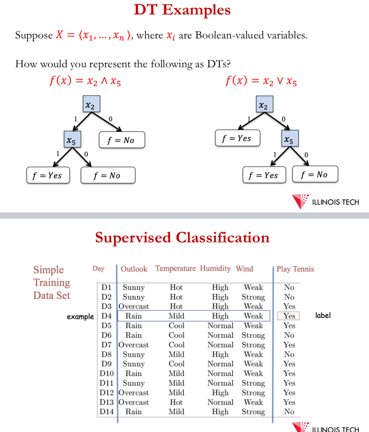
problem statement

input: training labelled examples (x_i, y_i) of unknown target function f

examples described by their values on some set of features or attributes

• (outlook = rain, temperature = hot, humidity = high, wind = weak)

unknown target function f: Z→ Y

• e.g. Y = {0, 1} label space

• e.g. 1 if we play tennis on this day, else 0

output: hypothesis h ∈ 𝐻 that (best) approximates target function f

• set of function hypotheses H = {h | f: X → Y}

• each hypothesis h is a d.t.

constructing a dt

how to automatically find a good hypothesis for training data?

• = algorithmic question, main topic of comp sci

when do we generalise + do well on unseen data?

• learning theory quantifies ability to generalise as a function of the amount of training data + hypothesis space

• Occam’s razor: use the simplest hypothesis consistent with data

short hypothesis that fits data = less likely to be a statistical coincidence, but it’s highly probable that a sufficiently complex hypothesis will fit the data

top-down induction

ID3 (iterative dichotomiser 3):

• Used to generate a decision tree from a dataset

• natural greedy approach to growing a decision tree using top-down approach (from root → leaves by repeatedly replacing an existing leaf with an internal node)

Algorithm:

• pick the best attribute to split at the root based on training data

• recurse on children that are impure (that have both yes + no)

ID3

greedy approach where we grow tree from root to leaves by repeatedly replacing an existing leaf with an internal node

node = Root

main loop:

1. A ← the best design attribute for next node

2. assign A as decision attribute for node

3. for each value of A, create new descendent of node

4. if training examples perfectly classifies, then STOP, else, ITERATE over new leaf nodes

best attribute → statistical measure info gain = how well a given attribute separates the training examples according to the target classification

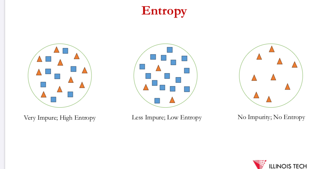
• in order to define info gain precisely → entropy = characterises the impurity of an arbitrary collection of examples

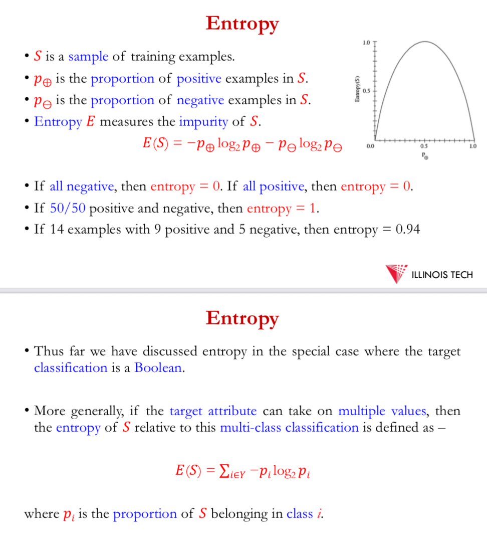
entropy

S = sample of training examples

𝑝⊕ = proportion of +ve examples in S

𝑝⊖ = proportion of -ve examples in S

Entropy 𝐸 measures the impurity of 𝑆.

𝐸(𝑆) = −𝑝⊕ log_2 𝑝⊕ − 𝑝⊖ log_2 𝑝⊖

if all -ve, entropy = 0, if all +ve, entropy = 0

• 50/50 , entropy = 1

• 14 examples w 9 +ve + 5 -ve = 0.94

above target classification = a Boolean

target attribute = multiple values = entropy of S relative to this multi-class classification

= 𝐸(𝑆) = ∑ _𝑖∈𝑌 −𝑝_𝑖 log_2 𝑝_𝑖

where 𝑝𝑖 is the proportion of 𝑆 belonging in class i.

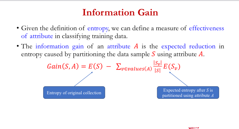
info gain

give definition of entropy, can define a measure of effectiveness of attribute in classifying training data

info gain of an attribute A = expected reduction in entropy caused by partitioning the data sample S using attribute A

𝐺𝑎𝑖𝑛 𝑆, 𝐴 = 𝐸 (𝑆) − ∑ _ 𝑣∈𝑣𝑎𝑙𝑢𝑒𝑠(𝐴) |𝑆𝑣|/|𝑆| * 𝐸(𝑆𝑣)

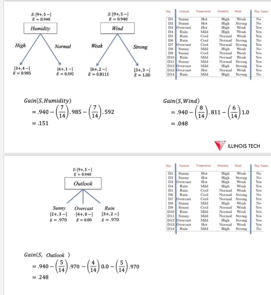
example

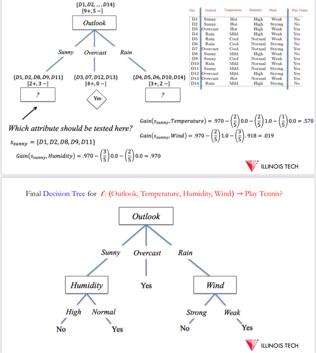
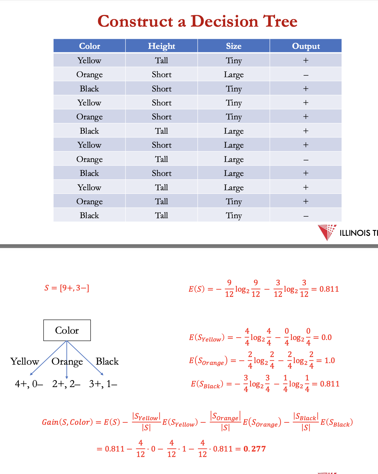
another example : constructing a decision tree

1. finding which feature to split on - choosing color as highest info gain

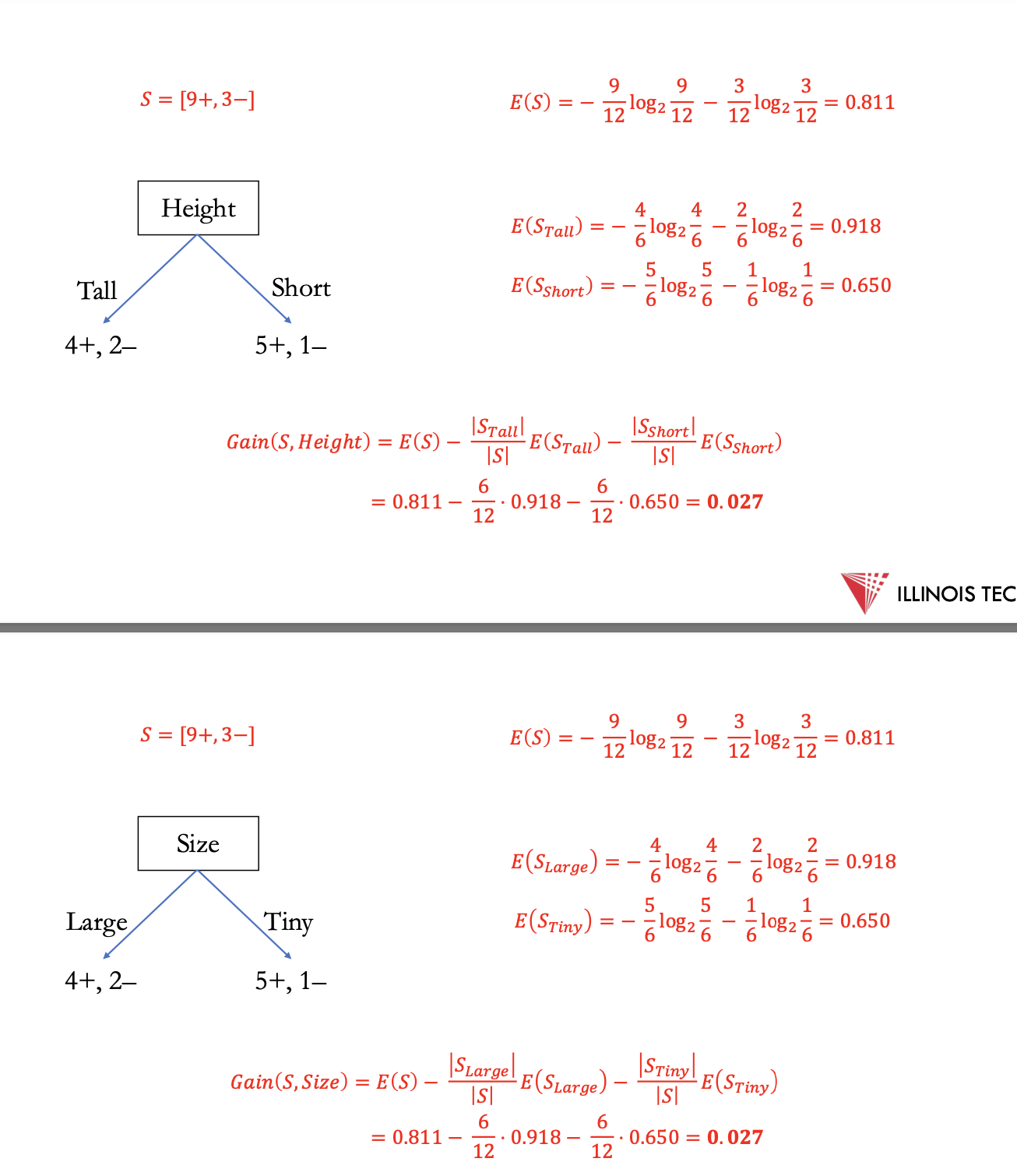
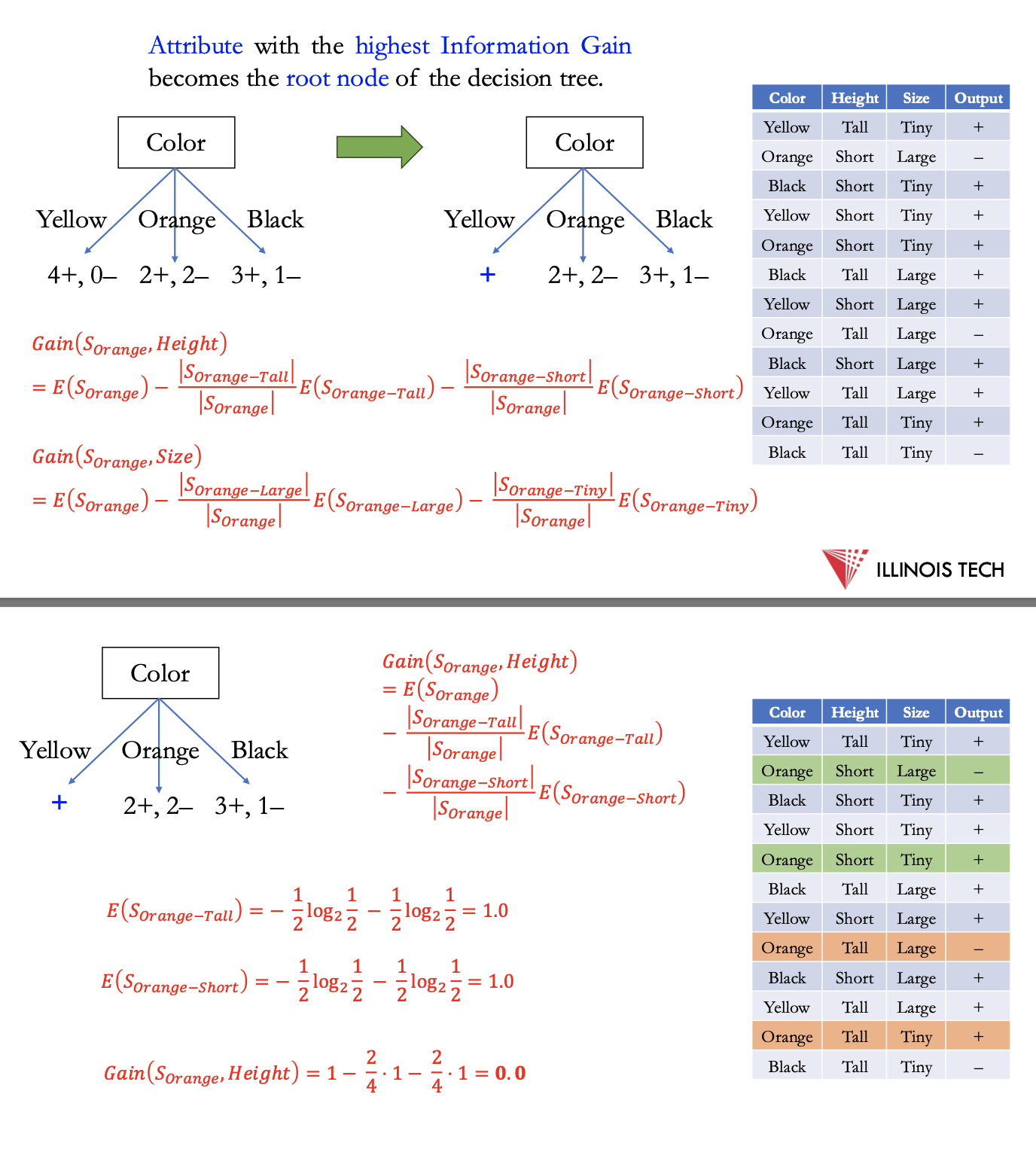
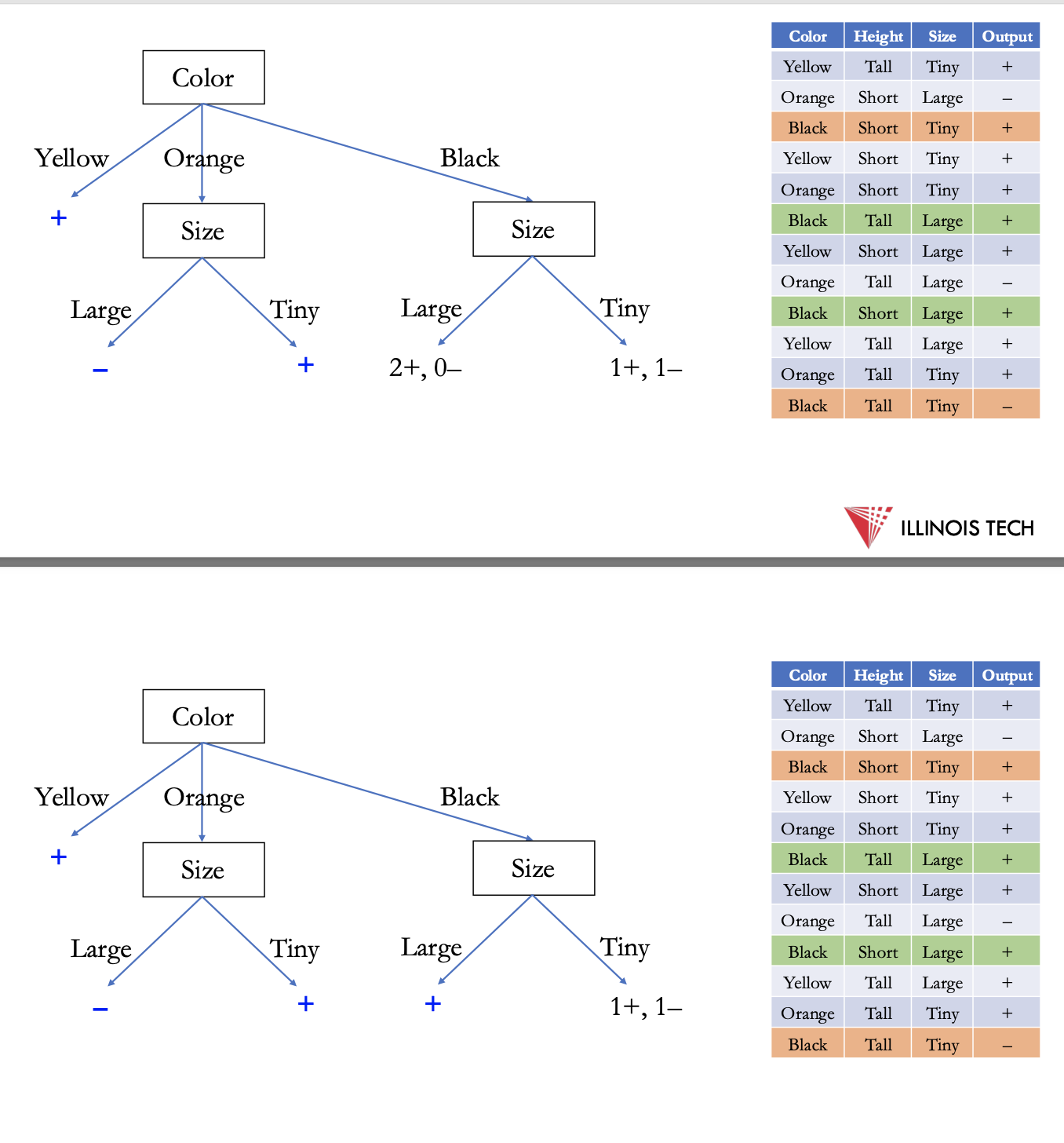
next for each new section calculate entropy, split on next highest feature

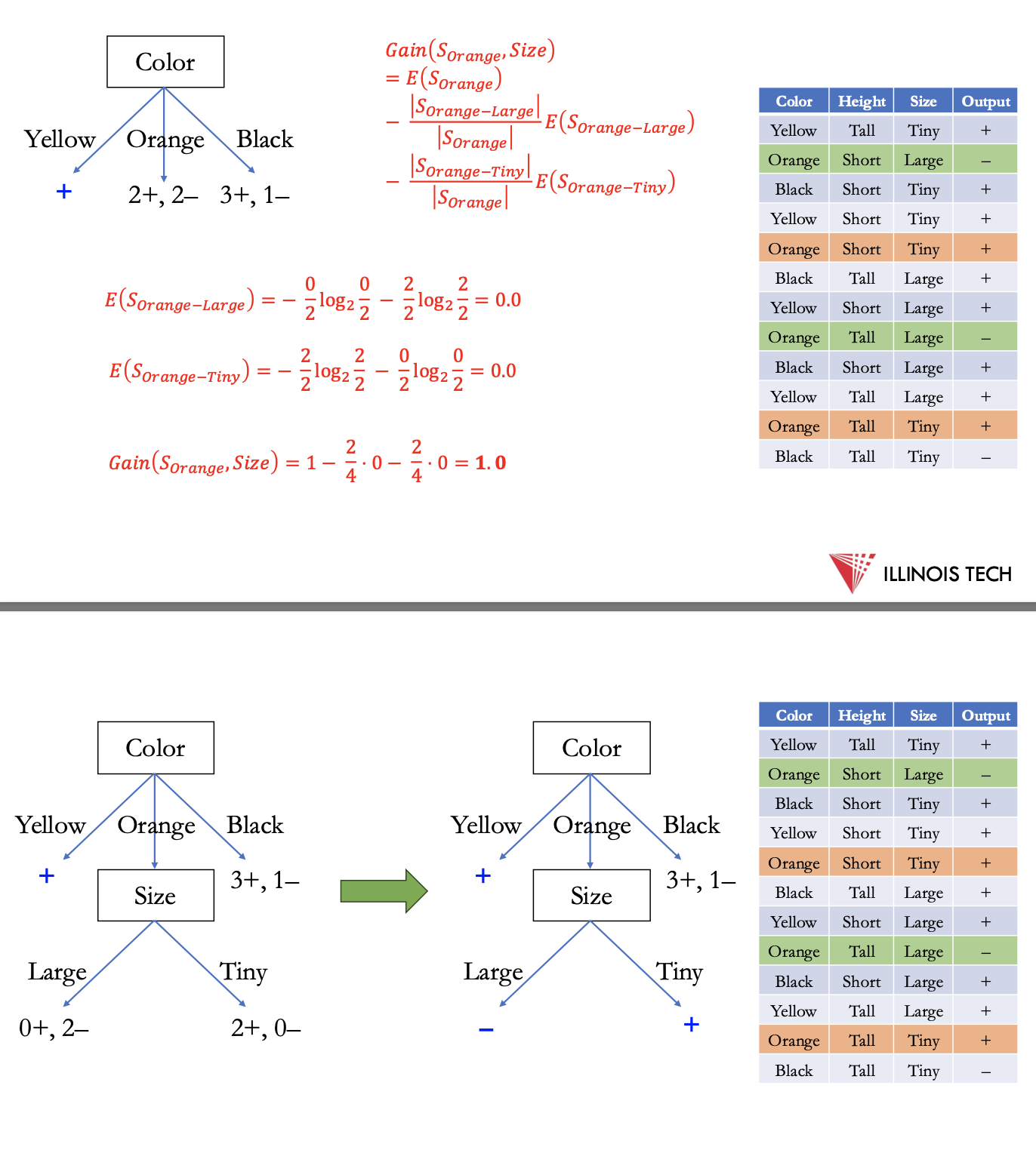
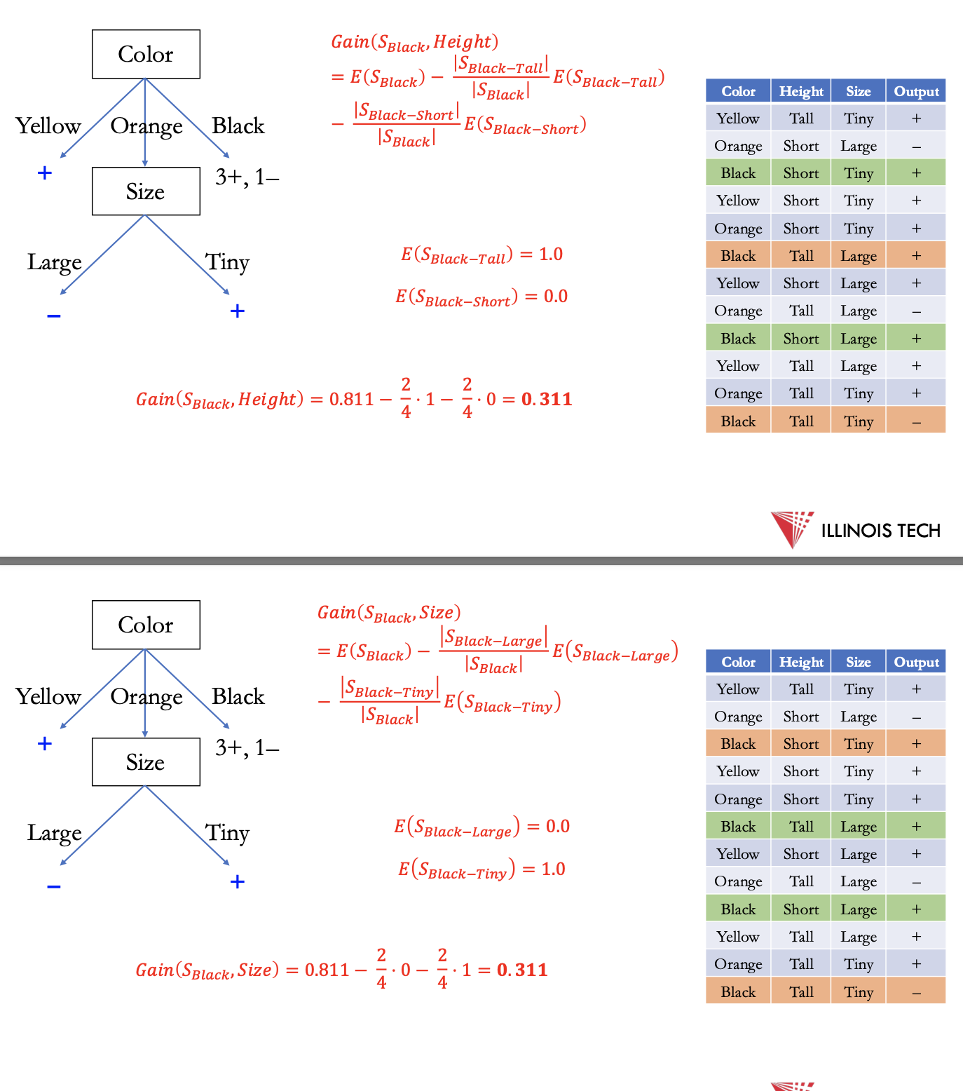
split black to size - still not fully pure → height for tiny

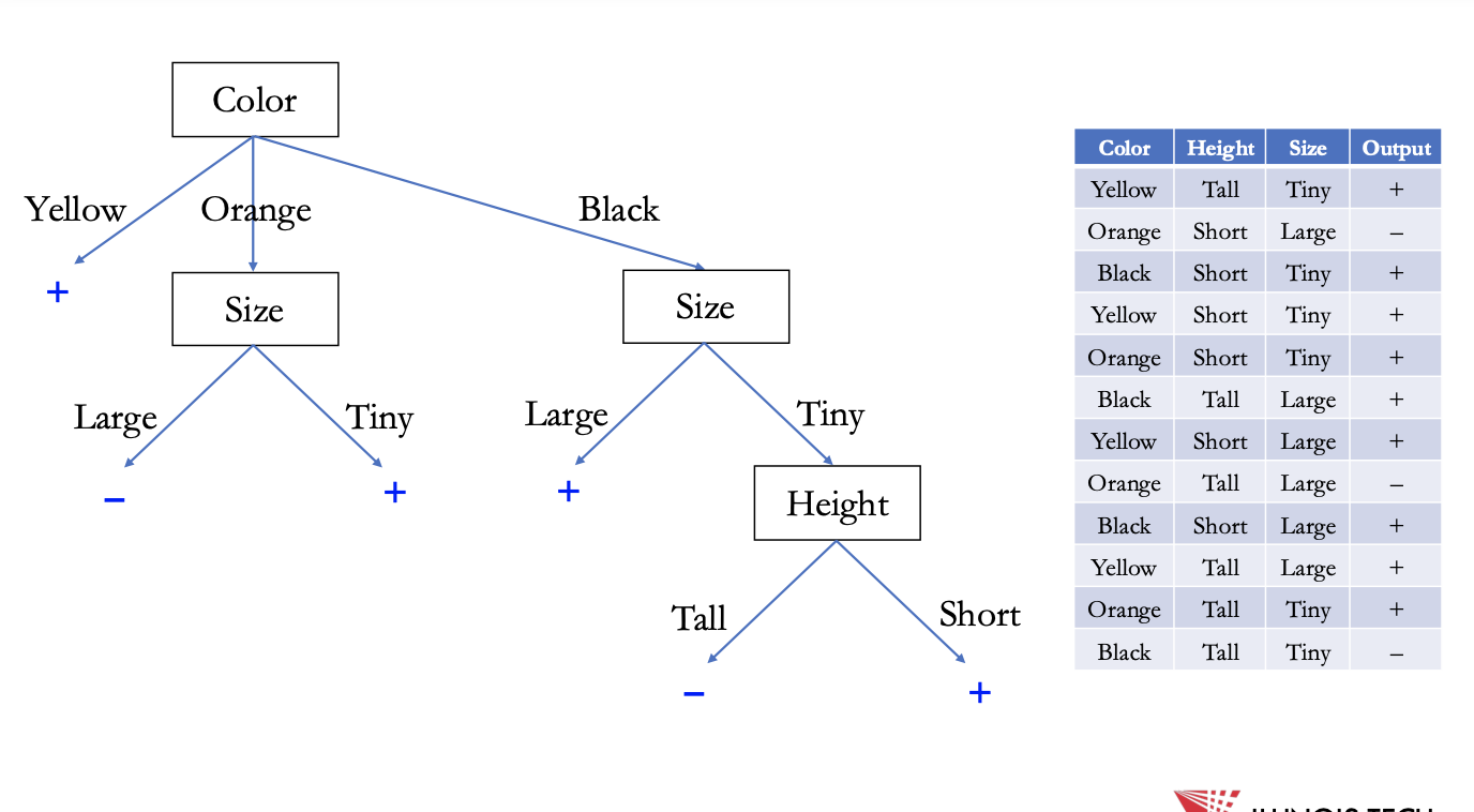
finished d.t.

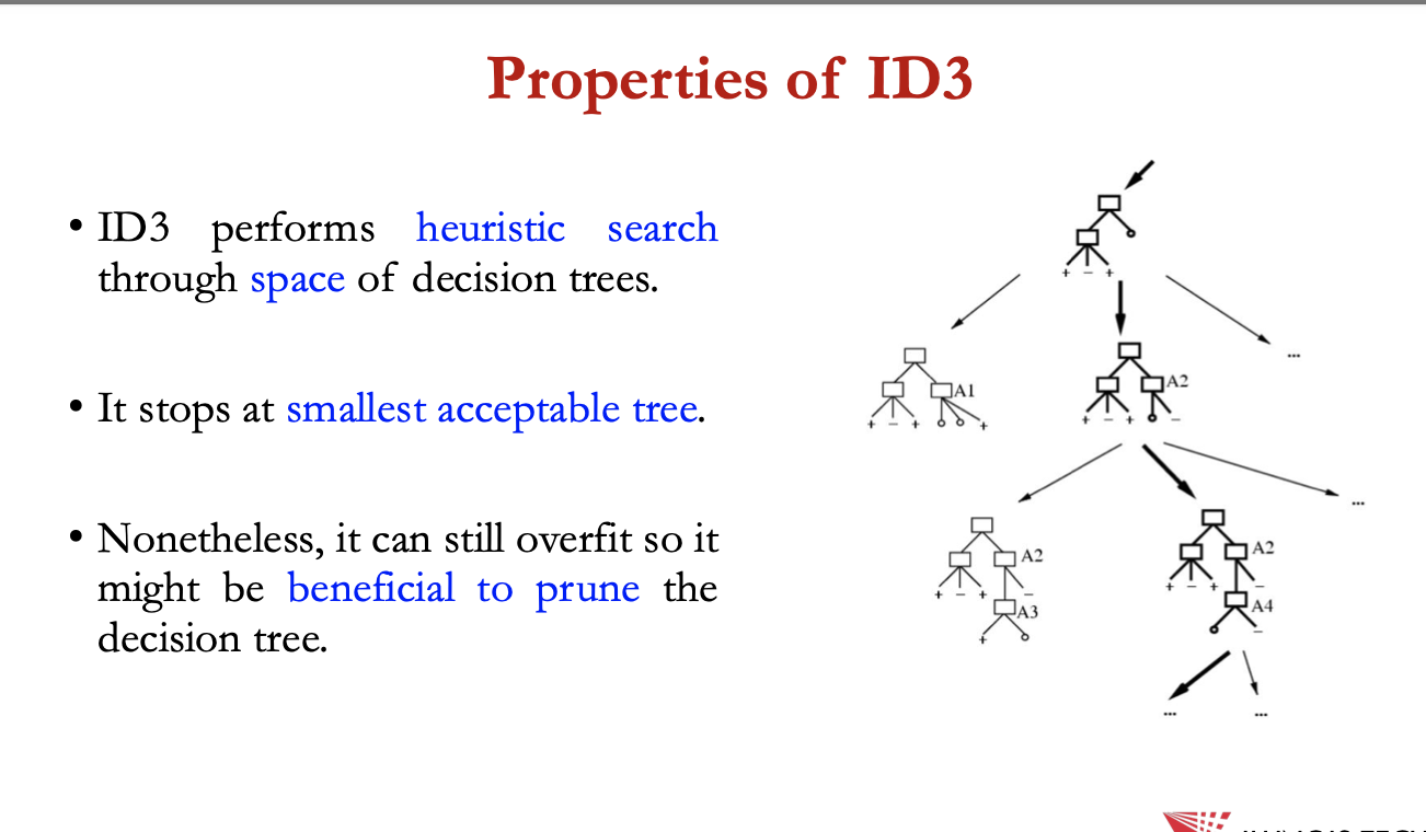
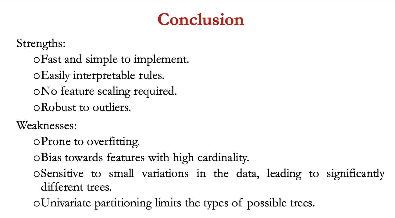
properties of ID3

ID3 performs heuristic search through space of decision trees

it stops at smallest acceptable tree

nonetheless, it can still overfit so it might be beneficial to prune the decision tree

overfitting

could occur bc of noisy data + bc ID3 isn’t guaranteed to output a small hypothesis even if one exists

avoiding overfitting:

1. stop growing when data split not statistically significant

2. acquire more training data

3. remove irrelevant attributes

4. grow full tree, then post prune

reduced error pruning

pruning a decision node consists of removing the subtree rooted at that node, making it a leaf node, + assigning it to the most common classification of the training examples affiliated with that node.

split data into training + validation set

do until further pruning = harmful:

1. evaluate impact on validation set of pruning each possible node

2. greedily remove the one that improves the validation set accuracy

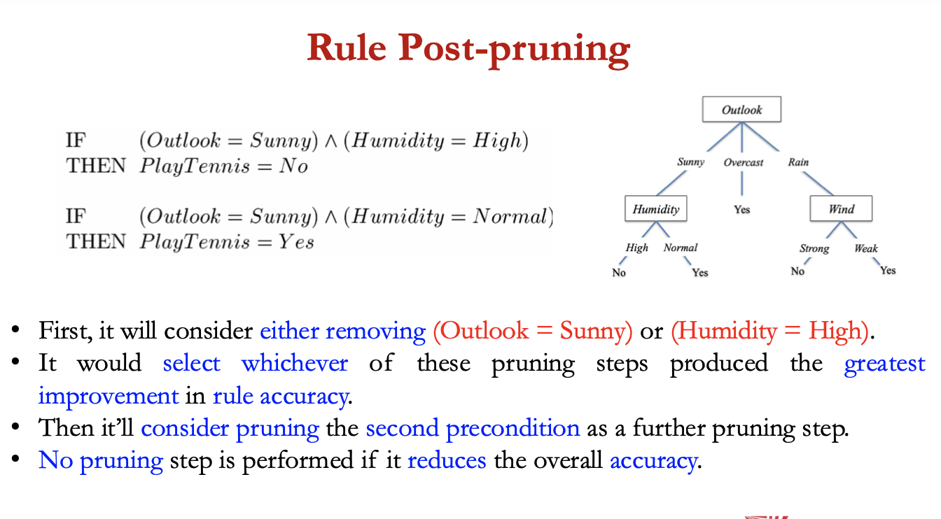
rule post pruning

1. infer the decision tree from the training set, growing the tree until the training data is fit as well as possible + allowing overfitting to occur

2. convert the learned tree into an equivalent set of rules by creating one rule for each path from root node to leaf node

3. prune each rule by removing any preconditions that result in improving its accuracy

• No pruning step is performed if it reduces the overall accuracy.

extensions to ID3

using gain rations

real valued data

noisy data + overfitting

C4.5 = extension of ID3 that accounts for unavailable values, continuous attribute value ranges, pruning of decision trees, etc.

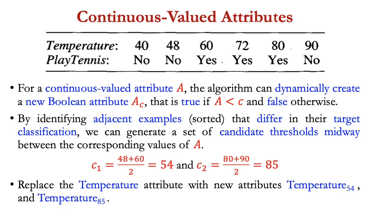
continuous valued attributes

for a continuous valued attribute A, the algorithm can dynamically create a new Boolean attribute A_c, that’s true if A<c and false otherwise

by identifying adjacent examples (sorted) that differ in their target classification, we can generate a set of candidate thresholds midway between the corresponding values of A

c₁ = (48+60)/2 = 54

c₂ = (80+90) /2

• replace temperature attribute with new attributes Temperature₅₄ and Temperature₈₅

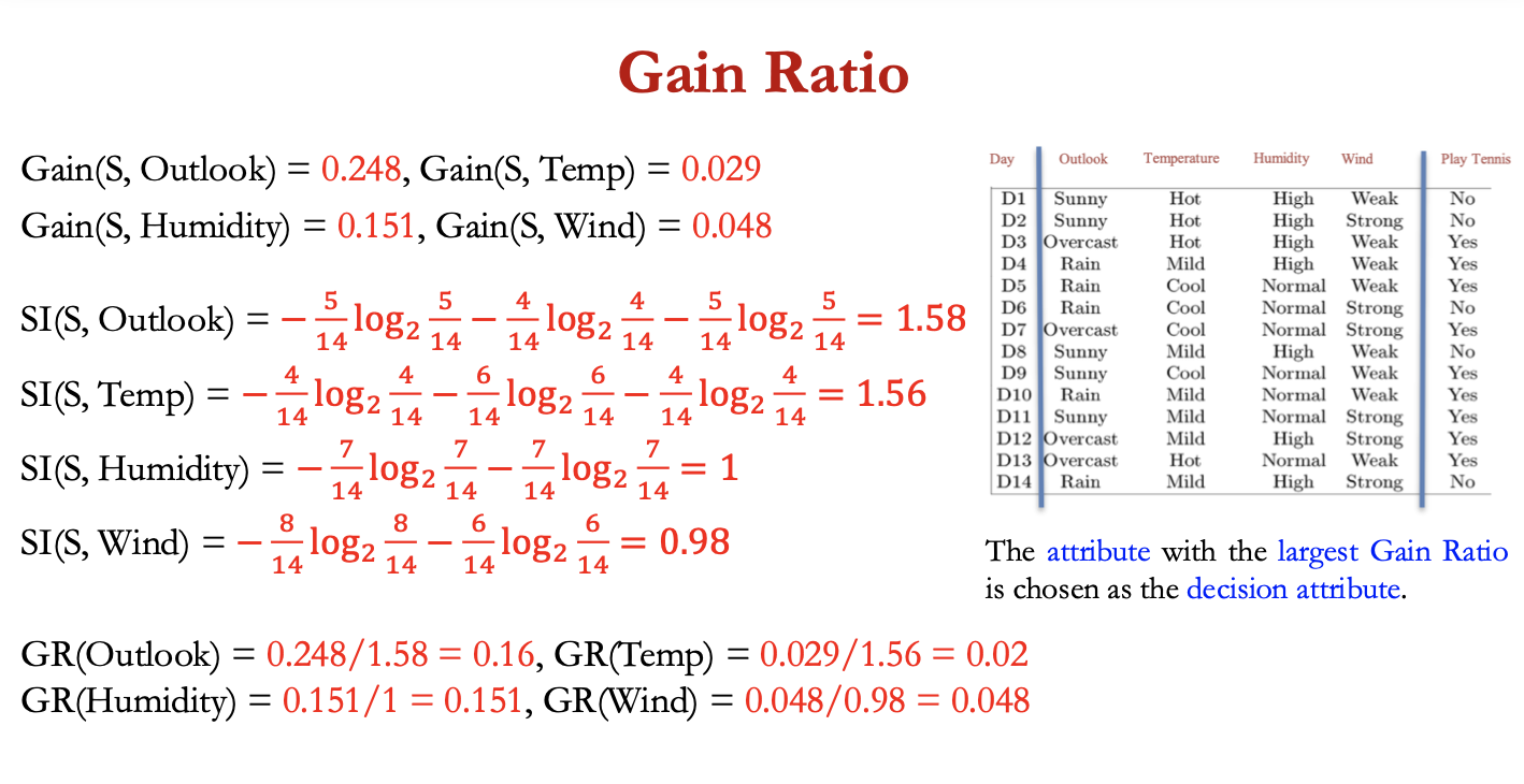
gain ratio

bias in Info Gain measure that favours attributes with many values over those with few values

gain ratio penalises attributes by incorporating a term, SplitInfo(S,A), that is sensitive to how broadly and uniformly an attribute splits the data

𝑆𝑝𝑙𝑖𝑡𝐼𝑛𝑓𝑜 (𝑆, 𝐴) ≡ − ∑_{𝑣∈𝑣𝑎𝑙𝑢𝑒𝑠} (A) |𝑆𝑣| / |𝑆| log ₂ |𝑆𝑣| / |𝑆|

gain ratio:

𝐺𝑎𝑖𝑛𝑅𝑎𝑡𝑖𝑜 (𝑆, 𝐴) = 𝐺𝑎𝑖𝑛 (𝑆, 𝐴) / 𝑆𝑝𝑙𝑖𝑡𝐼𝑛𝑓𝑜(𝑆, 𝐴)

attribute w highest gain ratio = choses as decision attribute

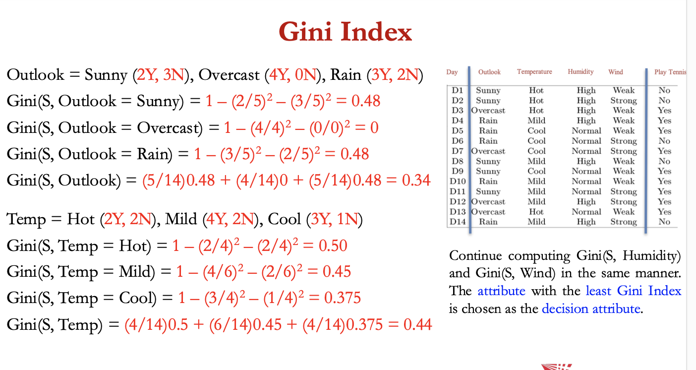
gini index

gini index measures the probability for a random instance of an attribute being misclassified when chosen randomly:

𝐺𝑖𝑛𝑖(𝑆, 𝐴) = 1 − ∑ _𝑖∈𝑌 𝑝_𝑖²

gini formula requires us to calculate the gini index for each sub node, then do a weighted avg to calculate gini index for the entire node.

𝐺𝑖𝑛𝑖(𝑆) = ∑ _{𝑣∈𝑣𝑎𝑙𝑢𝑒𝑠(A)} |𝑆𝑣| / |𝑆| 𝐺𝑖𝑛𝑖(𝑆, 𝐴)

the attribute w least Gini index = chosen as decision attribute

handling missing values

consider the situation in which Gain (S,A) is to be calculated at node n to evaluate whether attribute A is suited to be a decision node. Suppose, (x, c(x)) = training example and the value of A(x) is unknown

• one strategy for dealing with the missing attribute value = assign it the value that’s most common among training examples at the decision node n

• alternatively, we might assign it the most common value among examples at the decision node n that have the classification c(x)

2nd more complex procedure = assign a probability to each of the possible values A rather than simply assigning the most common value to the missing attribute A(x)

• these probabilities can be estimated based on observed frequencies of the various values for A among the examples at node n

e.g. a Boolean attribute A, if node n contains 6 known examples with A=1 and 4 with A=0, then we would say the probability that A(x) = 1 is 0.6, and the probability that A(x) = 0 is 0.4

• a fractional 0.6 of instance x is now distributed down the branch for A=1, and a fractional 0.4 of x down the other tree branch

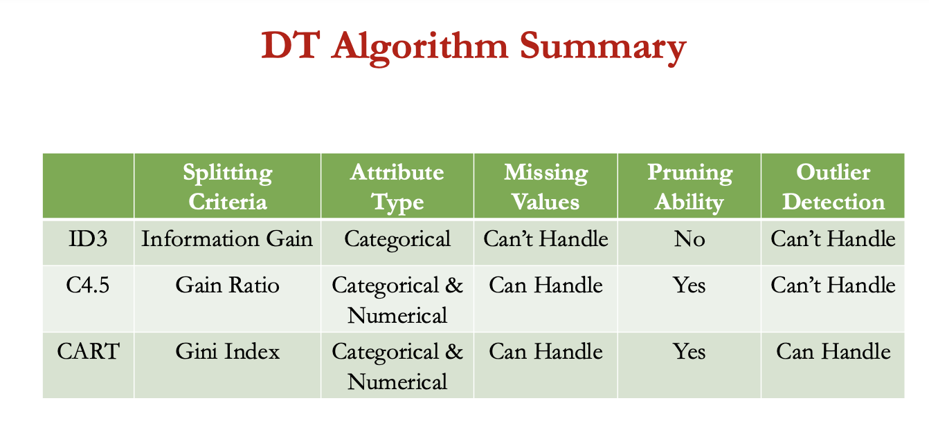
dt algo summary

when to use decision trees

feature importance: they’re helpful for identifying which input features are the most important in driving outcomes

explainability: their flowchart-like structure makes them intuitive + easy to understand, = valuable for explaining complex models to non-technical audiences

non-linear data: they’re particularly effective at handling data sets that don’t have a linear relationship between variables

use case scenarios:

• businesses use them to develop strategies + evaluate the cost effectiveness of options

• they provide a structured way to consider diff outcomes +  and probabilities for decisions, allowing for better risk management