Statistics 3 week 6

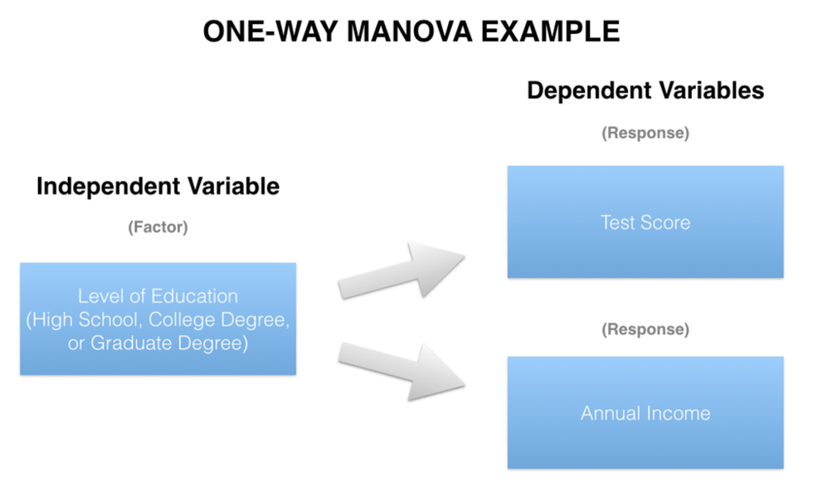
One-way MANOVA

One independent variable (factor) and two or more dependent variables (outcomes)

Two-way MANOVA

Two independent variables (factors and two or more dependent variables (outcomes)

Multivariate Analysis of Variance (MANOVA)

• For MANOVA (compared to ANOVA) at least one extra dependent variable is added to model.

• Goal of MANOVA is to test whether groups/conditions/cells differ for k different groups on a set of p different dependent variables.

• MANOVA takes into account possible correlations between dependent variables

Assumptions MANOVA

• Analogous to ANOVA but in multivariate setting:

• Extra 1: linear relationship between dependent variables (plot scatter plot matrix)

• Extra 2: no multicollinearity between dependent variables (calculate Pearson correlations) → No perfect correlation (over 0.9)

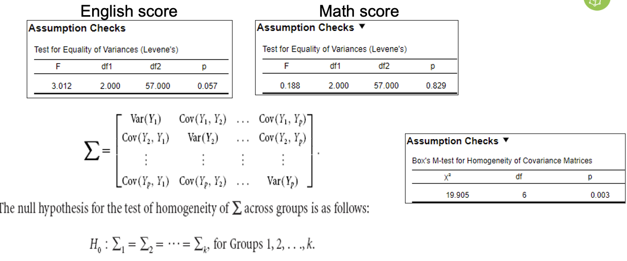
• Extra 3: equal variance-covariance matrices (perform Box’s M-test)

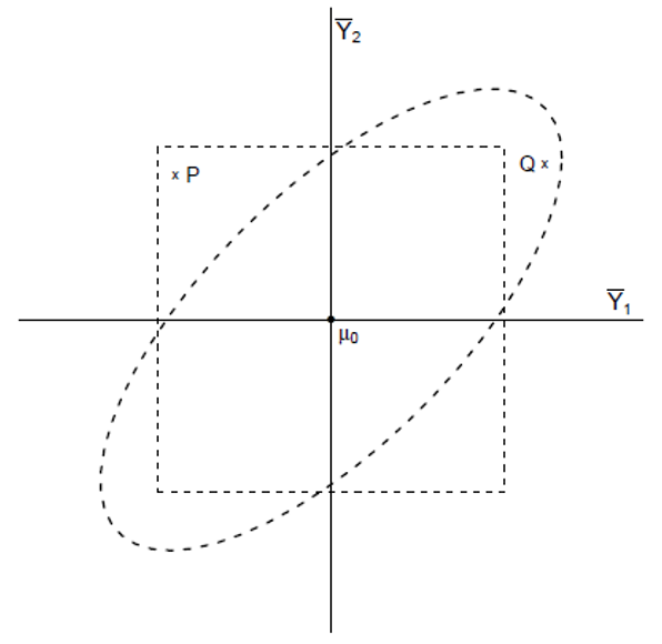
Univariate cs Multivariate testing

• The space outside the square is the rejection-area for two univariate tests (i.e., for at least 1 outcome the null hypothesis will be rejected).

  • With 2 univariate tests, multivariate H₀ is rejected if Y₁, Y_2,  or both fall outside the interval indicated by the square

  • Twice univariate testing assumes that both hypotheses are independent (orthogonal)

• The space outside the ellipse is the rejection-area for multivariate testing of 2 outcomes (i.e., for at least 1 outcome the null hypothesis is rejected).

  • When Y₁ and Y₂ are correlated (in this case positively), rejects null hypothesis less quickly if  (Y_1 ) ̅ are both relatively high (or low), compared to when deviations are opposed

Why not multiple ANOVAS?

• Type 1 error-problem with multiple testing:

  • “Running several univariate ANOVAs and reporting p different significance tests may result in an inflated risk of Type I error; a MANOVA provides a single “omnibus” test.”

• Taking into account possible relationship between Y’s:

  • “In MANOVA, each Y outcome variable is assessed while statistically controlling for inter-correlations with other Y outcomes; this makes it possible to assess the unique variance associated with each individual Y variable in the context of other Y outcomes.”

• Significant difference in patterns without individual significant differences:

  • “Sometimes an intervention effect can only be detected by examining the pattern of responses (there may be significant differences among groups in response pattern even if the individual Y variables considered in isolation do not differ significantly across groups).”

Assumption: equal variance-covariance matrices

• This MANOVA-assumption is the multivariate generalisation of the univariate ANOVA-assumption of equal variances:

  • Equal variances (SS: sum of squares) for each Y and equal covariances. The total of cross products is used. (SCP: sum cross products).

  • Box’s M Test for equal covariances is used with critical p-value: 0.001

  • In this example, this assumption thus does not seem to be violated.

Effect sizes MANOVA

• Most popular MANOVA-test statistic is Wilks’ Lambda (Λ)

  • The smaller, the larger the group effect

• With only one variable, Λ only uses the Sum of Squares

• That’s why the following effect sizes are used

  • Eta-squared

  • Partial Eta-squared

    • Where s is used for conversion-correction (not exam material)

Paradox for Box’s M-test and Levene’s test

• Both tests only have sufficient power with a relatively large N.

• However, unequal variances and covariances are mainly problematic for studies with a small N.

• In other words, for studies for which violating these assumptions is most problematic, it is hardest to decide whether the problem exists.

Other ANOVA-analyses that can be applied to MANOVA

• E.g.: contrasts to test for more complex hypotheses a priori.

• E.g.: pair-wise comparisons to get more post-hoc insights into where group differences exist.

MANOVA vs Repeated Measures ANOVA

• MANOVA: Multiple quantitative Y’s of different scales observed per subject,
  and qualitative X’s as predictor variables.

• Repeated measures ANOVA: Multiple quantitative Y’s of the same scale observed per subject, and qualitative X’s as predictor variables.

Advantages and disadvantages of repeated measures

• More measurements per observation, more info, subjects are their own control:

  • Filter out individual differences à focus on difference scores within subjects

  • For a specific required power, often fewer participants are needed

• Possible problem of carry over- and order-effects

• Specific equal variance-assumption for repeated measures:

  • Sphericity (ε): equal variances of differences between repeated measures. (Mauchly’s test)

Sphericity

• Sphericity in within-subject analysis is analogous to the equal variances-assumption in between-subjects ANOVA:

  • When the assumption is violated, the probability of a Type I-error increases (a lot).

  • Correction is possible by multiplying the number of degrees of freedom with epsilon (ε), which lies between 0 (no sphericity) and 1 (perfect sphericity):

    • Greenhouse-Geisser, Huynh-Feldt and Lower-bound are standard corrections given by SPSS

• Problem: Mauchly’s test for sphericity has low power for small samples (see above)