Lecture 7: Confidence Intervals 1: CLT, Intro to Statistical Inference, Estimates and Standard Errors, Interpretaion of Confidence

Feb 12, 2025 Yuan Fang, PhD

Random Sampling When

From one population to one sample

Random Sampling Why

Representative sampling

Random Sampling How

Inclusion/Exclusion criteria

Probability based sampling approaches:

• Simple random sampling

• Systematic sampling

• Stratified sampling

• Cluster sampling

• Multi-stage sampling

Random Sampling Results

Gives us confidence claiming something about the population based on what we found in the sample (confidence about our inference)

Randomization When

From one sample to two treatment groups

Randomization Why

Makes the treatment the biggest difference between the groups

Randomization How

Use probability-based method to separate samples into groups

Randomization Results

Gives us confidence that differences seen in the outcomes between the treatment groups at the end of the study are because of the differences in treatments

Central Limit Theorem Application

• Non-normal population

• Take samples of size n, as long as n is sufficiently large

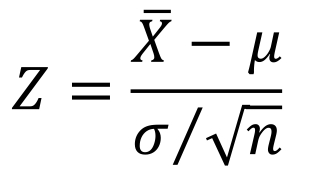
• The distribution of the sample mean is approximately normal, therefore can use Z-scores to compute probabilities

• We can then quantify the variability/uncertainty in the sample mean (estimate of the population mean)

• We get confidence intervals from this

• We get p-values from this

Central Limit Theroem

• The Central Limit Theorem

  • For any disribution, the sampling distribution of sample means becomes nearly normally distributed as the sample size grows

  • We will use the normal distribution to quantify uncertainty when we make inferences about a population mean based on the sample mean we take

• The sampling distribution of the means is close to Normal if either:

  • Large sample size if the population not normal

  • Population close to Normal

• Requirements

  • Independent (The CLT fails for dependent samples. A good survey design can ensure independence.)

  • Randomly collect sample

• Don’t confuse the distribution of the sample and the sampling distribution

Statistical Inference

• There are two broad areas of statistical inference: estimation and hypothesis testing

• Estimation - the population parameter is unknown, and sample statistics are used to generate estimates of the unknown parameter

• Hypothesis testing - an explicit statement or hypothesis is generated about the population parameter; sample statistics are analyzed and determined to either fail to reject or reject the hypothesis about the parameter

• In both estimation and hypothesis testing, it is assumes that the sample drawn from the population is a random sample

Estimation

• The point estimate is determined first. This is a sample statistic.

  • Best estimate of the true population parameter based on our data

  • The point estimates for the population mean and population proportion are the sample mean and sample proportion, respectively

• Calculating confidence intervals (or interval estimates) is the process of determining likely values for an unknown population parameter

• So, to find the Cl for the population mean or the population proportion, we start with the respective point estimate:

  • sample mean or the

  • sample proportion

• A point estimate for a population parameter is the “best” single number estimate of that parameter

• Confidence interval is a range of values for the parameter

point estimate ± margin of error

• A confidence interval estimate is a range of values for the population parameter with a level of confidence attached (e.g., 95% confidence that the range or interval contains the parameter)

  • Could be 90% or 99% or 98% or…

Interpretation

• Remember the truth that we are trying to estimate is fixed

  • So, we can NEVER say that there is a 95% chance or 95% probability the parameter is in the interval. The truth either is in out confidence interval or it is not. We WILL NOT assign a probability to it

  • This is why we ONLY use the word “confidence” and interpret from your perspective

• Interpreting confidence intervals: “I am 95% confident that between 45% and 75% students had flu shots in 2019

• OR

  I am 95% confident that the true proportion of students who had flu shots is between 0.45 and 0.75, or between 45% or 75%

Confidence Interval Estimates

point estimate ± margin of error

point estimate ± critical value x SE (point estimate)

• SE (point estimate) = standard error of the point estimate. This is the standard deviation of the sampling distribution

• Critical value comes from the percentiles of the sampling distribution for the sample statistic

  • It tells you the number of SEs needed for 95% (if constructing a 95% CI) of random samples to yield confidence intervals that capture the true parameter value

  • Critical value has to do with a level of confidence (90%, 95%, 99%, etc)

• The level of confidence reflects how likely it is that the CI contains the true, unknown parameter. It comes from the probabilities related to the sampling distribution

  • Remember, this is NOT the probability regarding the population parameter

CI for the population mean μ

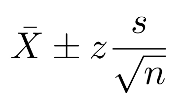
Higher confidence levels have larger z values, which translate to larger margins of error and wider CIs. For example, to be 99% confident that a CI contains the true unknown parameter, we need a wider interval

• We have used s instead of σ. If we know σ, we should use σ

• The above formula works OK when we have larger samples

• For smaller samples, if we are using 1.96 (from a normal distribution) for a 95% confidence level, we run into issues (this number is too small)

  • We need a new sampling distribution of the sample mean then

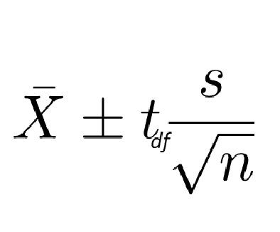
  • This is called the t-distribution

• Unless you know that the population is normally distributed or you know the true population standard deviation is σ, when constructing CIs for the population mean, use the t-distribution

• SKIN: standard deviation known is normal

• SUIT: standard deviation unknown is t

• CI for population proportion, the t-distribution is not used, always use normal

• The t distribution is another probability model for a continuous variable

• The t distribution takes a slightly different shape depending on the exact sample size

  • t distributions are indexed by degrees of freedom (df) which is defined as n - 1

  • If df = ∞, the t distribution is the same as the normal distribution

• It is important to note that the approximate use of the t distribution assumes that the variable of interest is approximately normally distributed

• Specifically, the t values for CIs are larger for smaller samples, resulting in larger margins of error

  • i.e., there is more imprecision with small samples

Really large sample size, or variable population normally distributed

Good default. Especially good for smaller sample size