Sticky prices and the NKPC

What is the problem with rational expectations?

It gets us immediate and costless disinflation with no central bank intervention required, which does not accord with existing theory.

What implicit assumption gives us this?

An implicit assumption has been that prices in goods markets are entirely flexible and that firms can always optimise their markup of prices over wages meaning any labour market out of equilibrium would operate on the PS curve.

What is Keynesian economics? What is the challenge with RE?

The model, with adaptive expectations, delivers two key characteristics of Keynesian economics. Firstly, the economy takes several periods to stabilise after a shock. Secondly, monetary policy plays an important role in stabilising the economy.

Rational expectations are the antithesis of Keynesian economics. A model featuring rational expectations and flexible prices is known as New Classical macro-economy.

In order to deliver Keynesian style results, while retaining rational expectations, new Keynesian economists dispensed with the idea of fully flexible prices and instead introduced sticky prices.

Why may firms keep their prices the same in the aftermath of a shock?

Firms may keep their prices the same in the aftermath of a shock because there is a deterrent to price-adjustment known as the menu-cost. For example, the physical or time cost from having to print new price labels and menus, edit catalogues, and advertise these price changes as well as the staff time you must devote to re-optimising the price in the first place. Changing prices unexpectedly is also detrimental to good will. If this menu cost is sufficiently high then it may dominate any short-term profit gains that the firm could secure by adjusting their prices. Levy et al.’s (1997) analysis found that menu costs, while not large, are far from trivial. For the average store in their sample, expenditures on changing prices amounted to between 0.5 and 1 percent of revenues.

What is the caveat to this?

However, modern technology has rendered basically all of these menu costs obsolete. Technology can help firms optimise the new price very easily, and then communicate this new price to customers quickly and at a low cost. Hence, it is unclear how small menu costs can account for the failure of prices to adjust when the economy is in recession and firms are facing losses.

What is the solution?

Ball, Mankiw and Romer (BMR) 1988 highlight how even trivial menu costs can prevent firms from optimising their prices, hence delivering the price stickiness which is central to New Keynesian analysis. They present a model of staggered price setting whereby small menu costs lead to individually rational firms not adjusting prices due to “aggregate demand externalities” imposed on them by other firms.

What is the BMR set up?

-            Imperfect competition amongst firms (a competitive firm will always vary prices after demand shocks).

-            Rational expectations.

-            Time contingent pricing: firms plan to re-set their prices at fixed intervals. For example, every 1^st January. If firms schedule their price adjustments, the marginal menu cost is effectively zero since the fixed cost of adjustment is already sunk. The incremental cost of responding to demand conditions at that moment is zero.

-            However, unscheduled price changes at any other time still involve a menu cost.

-            The final important assumption is that the scheduling of price adjustments for different firms are uniformly distributed across the year.

Show a firm’s price-quantity graph:

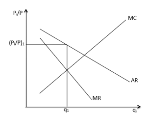
Show graphically and explain what happens in response to a negative demand shock with no menu costs:

Relative price (price of my good/general level of prices) on the y-axis. The firm produces q₁ where MR = MC.

In response to a negative demand shock, AR and MR shift leftwards for the firm. With no menu costs, the firm would simply re-equate MR with MC and reduce their price to achieve the relative price (p_i /p)₂. All other firms would do the exact same thing thus driving down the aggregate price level p.

The fall in p raises demand along the AD curve – as deflation leads to increased purchasing power and hence greater consumption - which then pushes AR’ and MR’ back up to the original AR and MR lines (since demand is higher without any change to relative prices given all firms acted the same). Thus, the original relative price is restored for all.

The important takeaway is that rational firms with no menu costs will end up stabilising the economy.

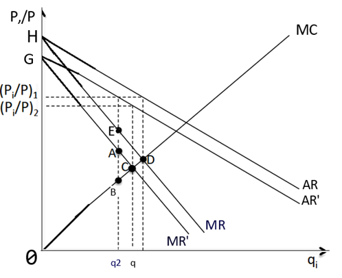
Now explain what happens with menu costs:

Assuming price adjustments are uniformly distributed, 1 in 12 firms will have no menu cost and therefore definitely vary prices. However, 11 in 12 firms have to assess whether the profits that could be realised through adjusting the price justify paying the menu cost.

Profits pre-shock equals the triangle (HD0)

If they do not vary the price, the quantity sold drops to q₂ where the sticky price meets the new demand curve. Profits after the shock is the trapezium area (GAB0). Therefore, the loss in profit is equal to the area (HDBAG).

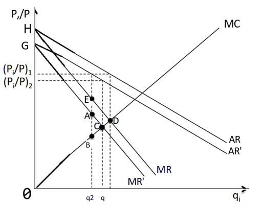
What is the key insight from BMR?

The key insight from BMR is that the menu cost does not need to exceed this lost profit region, which it likely never will. Instead, they divide this region into two separate components. Firstly, the private benefit of price adjustment (ABC) which is the incremental profit that a firm can realise as a result of that firm’s individual actions. They can decide to push up output from q₂ to q_c.

The area HDCG represents the aggregate demand externality: the profits that are externally conferred onto the firm by the price-cutting endeavours of all other firms in the economy (either from reduced interest rates or increased private sector purchasing power). These stabilising effects shift the AR and MR back to their original levels and confer this extra wealth.

What will firms do?

The argument from BMR is that the profit-maximizing firms will base their decision of whether to adjust prices based only on the private benefit of price adjustment. The aggregate demand externality cannot influence their decision as it has no relevance. When only looking at the private benefit of price adjustment (ABC), even a trivial menu cost could exceed this benefit. Thus, maintaining their fixed price is the rational choice.

What is the crucial thing we learn about price stickiness?

This BMR analysis shows that price stickiness is not derived simply by assuming menu costs, but rather from the impact of menu costs when the firm’s decision-making is skewed by an externality problem. Sticky prices are the result of a co-ordination failure as each firm ignores the benefits conferred by other firms’ price changes. If there existed a social planner in this economy, they would tell every firm to cut their price as such an adjustment would be welfare improving. As there is no device in reality to co-ordinate the actions of all these firms, these firms will only think about the private benefit of their adjustment.

When is price inertia most likely?

Menu costs are more likely to dominate whenever this ABC private-profit triangle gets squeezed, which occurs when the MC is relatively elastic. A flatter MC reduces the size of the private profit gain relative to the externally conferred gain. Factors contributing to a flat MC are known as real rigidities and include a relatively flat WS curve in the labour market (since labour costs then vary little with employment and output, and wages are a key element of the MC). These contextual factors exacerbate the effects of nominal rigidities such as menu costs.

What is another factor affecting price adjustment?

Another factor affecting price adjustment is labour market contracting. Firms do not renegotiate wages each period but employ workers on formal contracts that fix pay temporarily. Although such contracts may seem too short to generate prolonged rigidity, Romer (2006) emphasises the importance of implicit contracts: many jobs involve firm-specific skills and long-term relationships, so both firms and workers value the continuation of the match. Because employment decisions depend on expected lifetime income rather than just the current wage, cutting wages to clear the market can destroy valuable matches and morale. As a result, wages adjust slowly, marginal cost responds weakly to downturns, and price adjustment is muted.

What are the implications on the PC?

Recall that BMR have a constant fraction of firms undertaking a scheduled price change at any point in time and these firms always cut prices. Hence, there will always be some adjustment of aggregate prices (inflation) to accompany change in output i.e. a PC. If planned price reviews are more frequent then the PC will be steeper.

What determines the frequency of scheduled price reviews in an economy?

The history of inflation in that economy determines the frequency of scheduled price reviews. If a country has a history of high inflation, firms are disincentivized from scheduling long periods without price reviews and committing themselves to fixed prices. In support of this analysis, BMR present evidence that countries with higher historic inflation rates face a steeper short-run PC trade-off, which is consistent with their predictions.

Is menu costs the best explanation for price-stickiness?

While a consensus has emerged around sticky price macro models, it is far from clear that menu costs provide the best explanation for them. We have seen that menu cost frictions are most significant when there are real rigidities shaping the balance between the private and external benefits of price adjustment. However, real rigidities from elastic labour supply are rarely observed in practice and, in fact, microeconomic theory expects labour supply to be quite inelastic. Thus, the condition under which the menu-cost argument is most likely to succeed does not have either empirical or theoretical backing in practice.

What is another issue with these models?

Furthermore, these models fail if we conceptualize the menu cost as a largely fixed cost which does not depend on the magnitude of the price changes being implemented (which seems a fair assumption). If this is the case, then in the face of large, negative IS shocks – and hence large leftward shifts of AR and MR – the private profit triangle is going to enlarge greatly. If we are evaluating this to a menu cost that is fixed or largely fixed then firms will always want to adjust their prices. Therefore, models of price-stickiness based around menu costs seem to fail when looking at very large negative IS shocks.

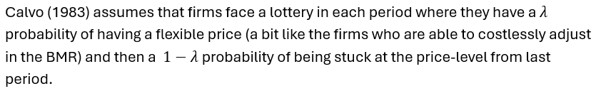
What does Calvo do?

What is the inflation rate and the inflation rate among flexible terms?

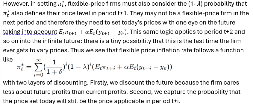
Expand on the inflation equation for flexible firms and explain why:

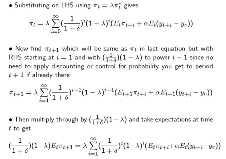
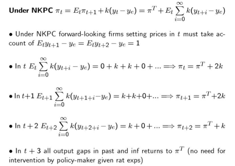
Derive the NKPC:

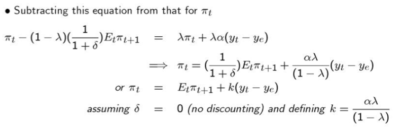
What does the NKPC tell us?

Inflation rate today is simply the expected inflation next period + the usual linear term multiplied by the output gap. This is the New Keynesian Phillips Curve (NKPC).

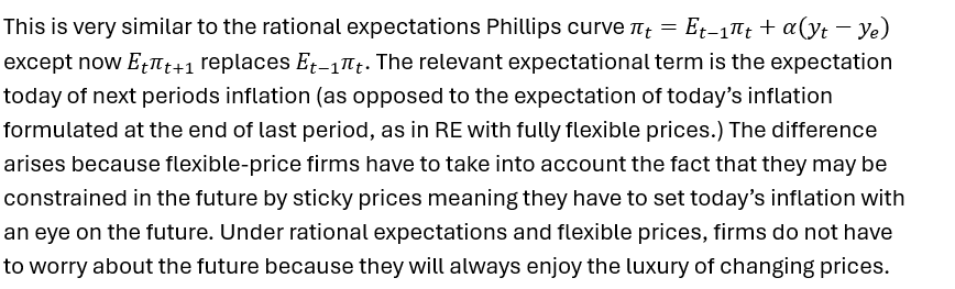
How does the NKPC differ from the REPC?

Derive the equivalent statement of NKPC:

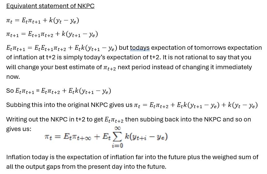
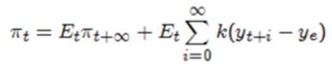
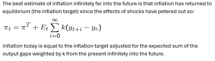
How can we simplify this further? What does the new equation tell us?

What happens under AEPC?

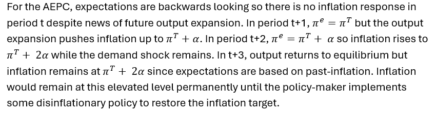
Why does this change for NKPC?

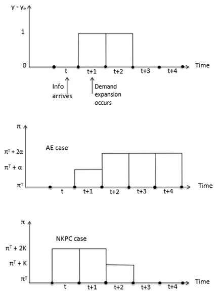
Under adaptive expectations, inflation is persistent and does not complete its full adjustment when the shock hits. Under the NKPC, there is no such persistence, and the economy performs its full inflation adjustment as soon as news of the shock arrives. This is because the flexible firms do not know if they will be a fixed-price firm in the future and therefore will adjust their prices immediately. Because firms are keeping an eye on the future, inflation adjusts up in period t before the increase in output has even kicked in.

Mathematically show what happens each period under NKPC?

Show the inflation over time for AE and NKPC respectively:

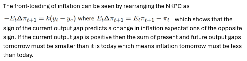
How can we capture the front-loading of inflation under NKPC?

Does the empirical literature support or undermine the NKPC?

Empirical literature on inflation typically finds evidence of inflation persistence, which supports the AEPC. Also, under AEPC a positive output gap is associated with rising inflation. In contrast, under NKPC there is a negative correlation between the output gap and changes to inflation which goes against the common observation that economic booms are periods of rising inflation. Thus, inflation dynamics that follow from the NKPC (which combines rational expectations and sticky prices) seem to be at odds with the inflation persistence and positive output-inflation trade-off seen in the data.

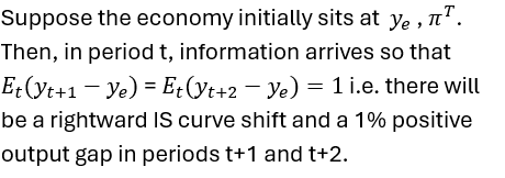
What if the output shock was unexpected and involved repeated surprises? (even after being surprised by higher output in t+1 agents still expect equilibrium output in t+2.)

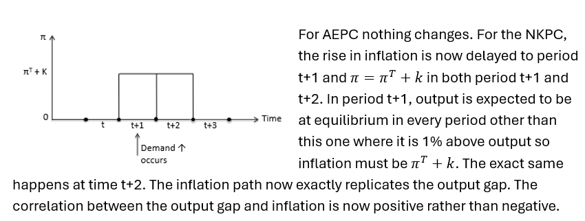
How does this support the NKPC?

Thus, the NKPC produces results more in line with empirical data when the shocks are unexpected. However, it is hard to interpret all movements in the data as the result of unexpected shocks.

What are hybrid Phillips curves?

Show the NKPC trajectory for a 1 period unexpected cost-push shock in in PC-MR space:

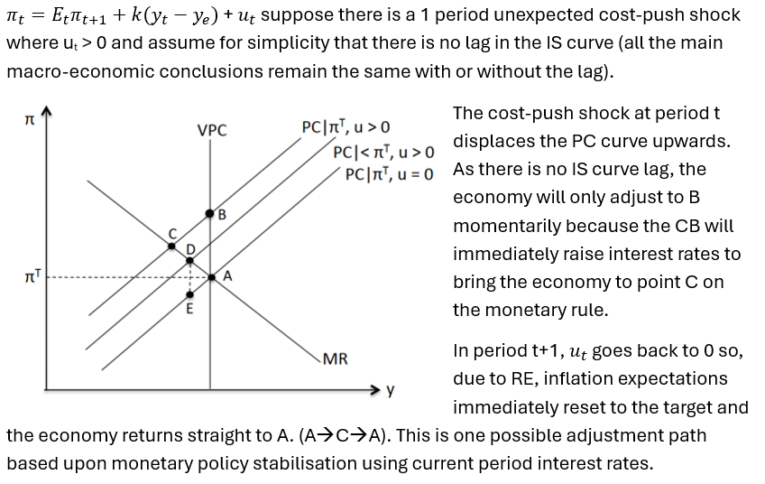
What is another possibility for the CB?

Another option for the CB is to issue forward guidance in period t pledging to set the real interest rates in period t+1 above the stabilising level. Absent of the IS curve lag, raising interest rates in period t+1 would have the effect of cutting output in period t+1 which would reduce the inflation rate. Rational agents know all this and will therefore revise down their expectations today of inflation in period t+1 causing us to intercept the VPC at a lower level in period t, helping us to achieve D rather than C.

Thus, the CB can either choose to vary current real interest rates (stabilising the economy by moving along the current PC) or by varying future inflation rates (shifting down the PC constraint).

What is the issue?

The disadvantage kicks in at period t+1. Unlike the first inflation path, the economy will not yet have returned to point A. If the CB pursues the forward guidance which they issue in period 1, output and inflation will have to fall in period t+1. This means the economy will be operating somewhere to the south-west of A, such as point E, where there is a higher value of social loss.

The second option is still preferred given the quadratic loss function as two smaller deviations from the bliss point is preferred to one large deviation. A policy of raising future interest rates therefore allows for more efficient stabilisation of the economy than a policy of raising current interest rates alone.

What happens if we extend this forward guidance?

We could extend the forward guidance. If the CB pledged to keep real interest rates high in period t+2, this would shift my PC down today bringing point D closer to point A and allowing even more efficient stabilisation of the economy. The downside is that we would not be at the bliss point by period t+2 but, again due to convex preferences, the CB would still be happy to engage in that strategy. Continuing this logic, the fully optimal policy will involve a very mild increase in interest rates in period t and then for this very mild interest rate to remain in place for an extended period before gradually bringing it back down to target.

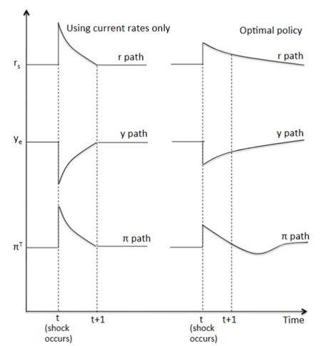
Compare the two options:

Using current interest rates only we get a severe but not persistent tightening of monetary policy. Under the optimal policy, we have a very mild tightening which eases off gradually over many periods. This gives us only a very shallow recession before output gradually returns to the optimal level. Inflation raises by much less due to the forward guidance and then is dragged back to the target, dipping below the target, before eventually recovering.

Show interest rates, output, inflation over time for the two options:

What is the issue with the optimal policy?

The issue is that the optimal policy is time-inconsistent. By period t+1, the optimal policy has delivered all of its benefits so it is no longer in the policymakers’ interests to pursue it now that only the costs remain. In t+1 the economy has in effect been stabilised so it is in the interest of the CB to revert on their forward guidance and set interest rates to the stabilising level to achieve point A.

However, a private-sector with rational expectations would understand this time-inconsistency and therefore see the forward guidance in period t as lacking credibility. With no way to credibly commit to the forward guidance, it would fall on deaf ears.

Summarise NKPC:

Therefore, while the NKPC opens up the possibility of a more efficient, optimal policy path, it is not implementable in practice. The only option is to fall back on the original policy of cranking up interest rates today and then reducing rates back to the stabilising level tomorrow.  This inefficiency is known as the stabilisation bias.

How can we make the optimal policy time-consistent?

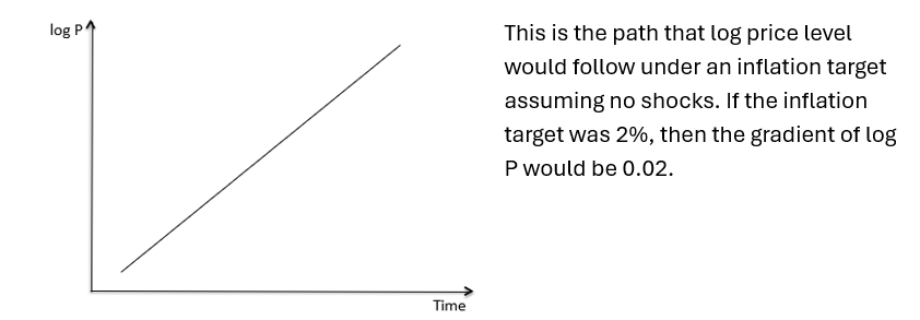
The optimal policy could be made time consistent, and therefore implementable, if we changed the mandate of the CB away from a simple 2% inflation target towards a price path target consistent with 2% inflation.

Show PPT graphically:

Show the original response and new response to a positive cost push shock on the graph:

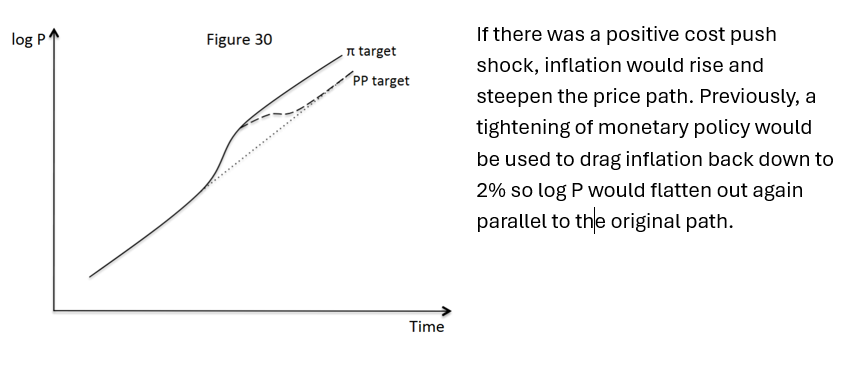
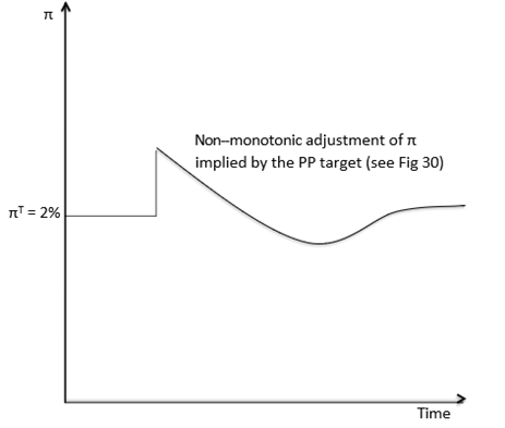
Explain what happens under PPT and why it solves the time inconsistency problem:

Under price path targeting, however, the CB has to drive the price path back down towards the counterfactual path that would have applied if the shock had never occurred in the first place. In order to restore the old trajectory, the CB would have to force inflation below 2% for some period in order to compensate for the previous overshoot of the inflation target. This entirely matches the path which inflation has to follow under optimal monetary policy, so this optimal monetary policy is now time-consistent. The CB now actively prefers point E to point A in period t+1 because its price path mandate now requires corrective action after a shock. Price-path targeting changes the incentives of the CB to deliver the exact non-monotonic inflation adjustment that is required by the optimal monetary policy. The issue of time-inconsistency and the associated stabilisation bias is overcome.

Show inflation over time:

Will rational expectations make output and inflation more stable in the face of shocks?

-            It depends on the model. Rational expectations can give us costless disinflation under the REPC model. However, inflation may jump around under the NKPC model, making output and inflation even less stable.

-            Does stability mean a quick return back to equilibrium, or does it mean a small change in inflation in every period? A protracted period of inflation being above target or output below equilibrium may be considered more “stable” than having inflation fluctuate around rapidly, even if the latter reaches equilibrium quicker. While under the AEPC inflation and output are disequilibrated for a long period of time, the adjustment process is smooth and gradual.

2014 Essay: “The more rapidly inflation adjusts the shorter booms and recessions will be.” Discuss different circumstances in which this may or may not be true.

-            Just because inflation adjusts doesn’t mean that booms and recessions may be shorter. For instance, under the NKPC model, inflation adjusts but booms and recessions are just as long. Or the central bank might intervene to make booms and recessions even more protracted (but milder). This means less pronounced but more persistent movements in interest rates, output and inflation.

2015 Part A: According to the New Keynesian Phillips curve, a one unit increase in the output gap relative to the previous period may be associated with either a rise in inflation relative to the previous period, no change in inflation relative to the previous period, or a decline in inflation relative to the previous period. Provide examples to illustrate each of these cases.

1.       An unexpected positive demand shock will cause an increase in output gap and inflation.

2.       No change: a shock that is known to last two periods arrives in time t, and we are now at time t+1 (the second period of the shock). Already priced in – so no change in inflation.

3.       Decrease: a positive demand shock was supposed to be 2 units, but is in fact only 1 unit. Inflation decreases.