Midterm 1

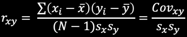
Correlation

• how two variables covary in relation to each other

  • how they move together/vary together

• standardized covariance

• the value of r can range between -1 and +1

  • - = move in opposite directions

  • + = move in the same directions

• if r = 0 — there is no linear relationship between the two variables

• the closer r is to ± 1, the stronger the relationship

• if r = ±1 — there is a perfect linear relationship between the variables

Deviation from the Mean

• Observation - mean = distance of the observation from the mean

Two ways to define correlation coefficient

• z scores

• covariation

z scores

• z = 0 — score = mean

• z > 0 — score ≠ mean

• z = 1 — score = 1 SD from mean

• z = 1 — score = 2 SD from mean

Variance Formula

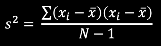
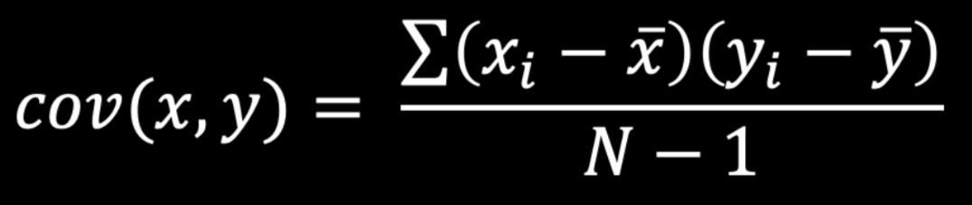
Covariance Formula

Coefficient Determination

• r² indicates the percent of the variability in y that is accounted for by the variability in x

Model

• variability in scores that we can account for

Error

• variability in scores that we cannot account for

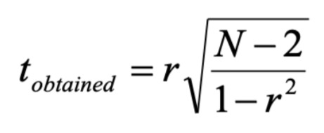
t obtained formula

Steps in Finding Correlation

1. create H0 and H1

2. set parameters (find critical t)

3. calculate t obtained

4. compare critical t and t obtained

5. find p-values in SPSS

Steps in Finding Confidence Intervals

1. convert Pearson’s r to z score

2. compute a confidence interval for z score

3. convert z score back to Pearson’s r

Calculating Confidence Intervals

• CI = value ± (z critical (SE))

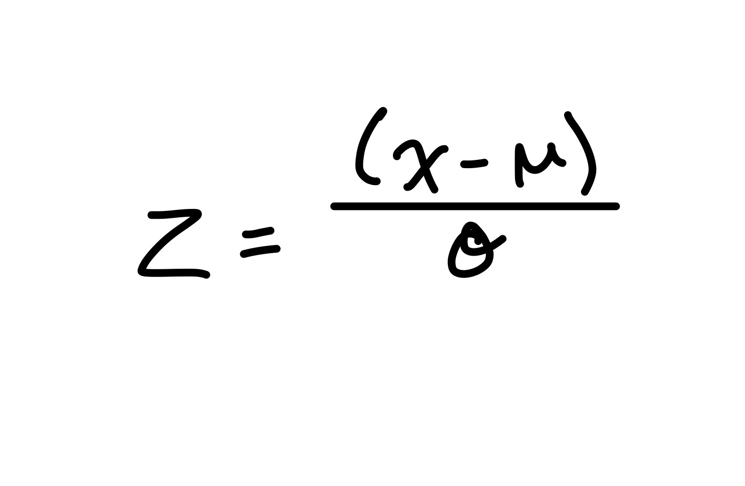
Standardization Formula

Reliability

• in research, the term reliability means “repeatability” or “consistency”

• a measure is considered reliable if it would give us the same result over and over again (assuming that what we are measuring isn’t changing!)

Internal Consistency Reliability

• AKA “coefficient alpha”, “Cronbach’s alpha”, “reliability coefficient”

• judge the reliability of an instrument by estimating how well the items that reflect the same construct yield similar results

• looks at how consistent the results are for different items for the same construct within the scale

  • questionnaires often have multiple questions dedicated to each factor (some need to be reverse coded)

Purpose of Internal Consistency Reliability

• used to assess the consistency of results across items within a test

• how well do the items “hang” together?

• typically, a reliability analysis is done on items that make up a single scale (items all supposed to measure roughly the same construct) — founded on correlations of items

Reliability Coefficients

• range from 0-1.00 with higher scores indicating the scales is more internally consistent

• generally, reliabilities above .80 are considered acceptable for research purposes

• reliability analyses are carried out on items AFTER recoding (reverse coding)

Validity

• is the test measuring what it claims to measure

Assumptions of Tests Based on Normal Distribution

• additivity

• normality of something or other

• homogeneity of variance/homoschedasticity

• independence

Additivity

• outcome = model + error

  • model used to predict variability

• the outcome variable (DV) is linearly related to any predictors (IV)

• if you have several predictors (IVs) then their combined effect is best described by adding their effects together

• if this assumption is met then your model is valid

Normally Distributed Something or Other

• the normal distribution is relevant to:

  • parameter estimates

  • confidence intervals around a parameter

  • null hypothesis significance testing

When does the Assumption of Normality Matter?

• in small samples

  • the central limit theorem allows us to forget about this assumption in larger samples

• in practical terms, as long as your sample is fairly large, outliers are a much more pressing concern than normality

Spotting Normality

• we don’t have access to the sampling distributions so we usually test the observed data

• central limit theorem

• graphical displays

Spotting Normality with the Central Limit Theorem

• if N > 30, the sampling distribution is normal anyway

Spotting Normality with graphical displays

• can use histograms or P-P Plots

P-P Plots

(probability-probability)

• when it sags: kurtosis is an issue

• when it forms an “S”: skewness is an issue

Values of Skew/Kurtosis

• 0 in a normal distribution

• convert to z (by dividing value by SE)

  • value greater than 1.96 = significantly different from normal

  • should be used for smaller sample sizes, if at all

Kolmogorov-Smirnov Test

• tests if data differ from a normal distribution

  • significant = non-normal data

  • non-significant = normal data

*for large sample sizes

Shapiro-Wilk Test

• tests if data differ from a normal distribution

  • significant = non-normal data

  • non-significant = normal data

*for small sample sizes

Homoschedasticity

• measuring variance of errors

  • variance of outcome variable should be stable across all conditions

Homogeneous

• uniform error rate across categories

Heterogeneous

• difference in error rate across categories

  • violation of homoschedasticity

Independence

• observations are completely independent from each other

  • violation example — 2 participants talk and share notes between the first and second parts of a test so their scores are no longer independent and now have a correlation

Violation of Assumptions of Independence

• grouped data

Violation of Assumptions of Normality

• robustness of test

• transformations

Violation of Assumptions of Homogeneity

• robustness and unequal sample sizes

• transformations

  • if you have not normal data, one way to make data normal is to conduct a transformation

Types of Transformations

• logarithmic transformation

• square root transformation

• reciprocal transformation

• arcsine transformation

• trimmed samples

• windsorized sample

Transformations

• always examine and understand data prior to performing analyses

• know the requirements of the data analysis technique to be used

• utilize data transformation with care and never use unless there is a clear reason

Square Root Transformation

• help decrease skewness and stabilize variances (homoschedasticity)

Reciprocal Transformation

• reduces influence of extreme values (outliers)

Arcsine Transformation

• elongates tails (good for leptokurtic distributions)

Trimmed Samples

• not really a transformation

• fixed value of extreme values you cut off

Windsorized Samples

• similar to trimmed samples

• extreme values replaced by values that occur at 5% in the tails

Steps in Hypothesis Testing

1. formulate research hypothesis

2. set up the null hypothesis

3. obtain the sampling distribution under the null hypothesis (choosing number of participants: past literature, power analysis)

4. obtain data; calculate statistics

5. given the sampling distribution, calculate the probability of obtaining a value that is as different as the one you have

6. on the basis of probability, decide whether to reject or fail to reject the null hypothesis

When do you reject the null hypothesis

• significance levels

• conventional levels

• the score that corresponds to alpha = critical value

  • if p < alpha, reject H0

  • if p > alpha, fail to reject H0

• the smaller the alpha, the more conservative the test (we are more likely to conserve H0)

Directional hypothesis

• indicates a direction (ex; time spent in class increases mind wandering)

• use a one tailed test

Nondirectional hypothesis

• does not indicate a direction (ex; time spent in class could increase or decrease mind wandering)

• use a two tailed test

Type I Error

• your test is significant (p < .05), so you reject the null hypothesis, but the null hypothesis is actually true

Type II Error

• your test is not significant (p > .05), you don’t reject the null hypothesis but you should have because it’s false

True or False — A significant result means the effect is important

• False

  • just because it is statistically significant does not mean it is actually significant in the real world

True or False — A non-significant result means that the null hypothesis is true

• False

  • tells us only that the effect is not big enough to be found with the sample size we had

  • fail to reject the null — doesn’t mean the effect is not there, just means you didn’t find it

True or False — a significant result means that the null hypothesis is false

• False

  • not a distinct yes or no, probabilistic reasoning — only 95% confident

True or False — The p-value gives you the effect size

• false

  • we need to do some further calculations to find effect

True or False — The population parameter (μ) will always be within a 95% confidence interval of the sample mean

• false

  • it’s an estimate

True or False — The sample statistic (M) will always be within a 95% confidence interval of the mean

• True

  • we calculate the confidence interval based on the sample mean so it is always right in the middle

Trends to Circumvent Problems with NHST

• effect size calculations — standardized so we can compare

• confidence intervals

Outcome = __________

(model) + error

• outcome — dependent variable

• model — independent variables

B₁

Slope

• increase in y for every increase in x

B₀

y-intercept

• y when x is 0

Parameter Estimates

• different samples drawn from the same population will likely yield different values for the mean

Sampling Error

• the difference between my sample and the population value

Sampling error formula

Interval Estimates using σ

• 95% confidence interval

  • lower limit: M + [z(critical)σ_M]

  • upper limit: M + [z(critical)σ_M]

Standard Error of the Sampling Distribution of Means

• used when we don’t know σ

Standard Error of the Sampling Distribution of Means Formula

Interval Estimates without σ

• 95% confidence interval

  • lower limit: M + [t(critical)SE_M]

  • upper limit: M + [t(critical)SE_M]

z scores vs. t scores

• z scores

  • σ is known

  • large sample sizes

• t scores

  • σ is not known (we introduce more error with SE_M when σ is not known and t corrects for this)

  • small sample sizes

t critical

• t[critical] = t(n-1)

t critical table

• degrees of freedom = n-1

  • then find percentage

The mean is sufficient whereas the mode is not (true or false)

• depends

  • mode is more appropriate for income

One should always plot data (true or false)

• true

Standard error is a measure of variability (true or false)

• false

  • estimate of variability across samples (standard deviation is a measure of variability)

You can compare standard deviations across samples (true or false)

• true

An outlier is a score that falls 3 standard deviations from the mean (true or false)

• true (usually)

  • this is the most common but it is subjective

Describing and Exploring Data Objectives

• to reduce data to a more interpretable form using graphical representation and measures of central tendency and dispersion

  • data description and exploration, including plotting, should be the first step in the analysis of any data set

Why Plot Data?

• gives a quick appreciation of the data set as a whole

• readily gives information about dispersion/spread and the distributional form/shape

• clear identification of outliers (if there’s one outlier we might want to go in and find out why)

• what might cause an outlier?

  • someone with an already high baseline for what you’re measuring (high stress levels make them more/less reactive to something)

What is an outlier?

definitions vary

• a data point that is far outside the norm for a variable or population and exerts undue influence

• values that are dubious in the eyes of the researcher

Fringeliers

• unusual events that occur more than seldom

  • not quite 3 standard deviations away from the mean to be considered outliers but still unusual

Reasons for Outliers

• data entry or measurement error

• sampling error

• natural variations

• response bias

Bar Chart

• has spaces between the bars (categorical data)

  • spaces used to distinguish between clear cut categories

Histogram

• no spaces between the bars (continuous data)

  • scores represent underlying continuity 

    • frequency chart of distribution

Point Estimators / Measures of Central Tendency

• mean

• median

• mode

Properties of Estimators

• sufficiency

• unbiasedness

• efficiency

• resistance

Sufficiency

• uses all the data

  • ex; mean

Unbiasedness

• approximates the population parameter

Efficacy

• low variability from sample to sample (sample population)

Resistance

• resistant to outliers

  • ex; median

Mode

• represents the largest number of people

• easy to spot

• unaffected by extreme scores (resistant)

• can be used for nominal, ordinal, interval, or ratio data

*distributions can have more than one

Median

• relatively unaffected by extreme scores (resistant to outliers)

• relatively unaffected by skewed distributions

• can be used with ordinal, interval, or ratio data

*sometimes not an actual score from the distribution

Mean

most common

• can be manipulated algebraically

• unbiased, efficient, and sufficient

• assumes continuous measurement (can only be used with interval and ratio data)

• minimizes sum of square deviations from it

  • gives smallest sum of squares of all methods

  • good estimator

• influenced by outliers

• influenced by skewness

Four Moments in Statistics

• Mean

• Variance

• Skewness

• Kurtosis

Mean Formula

Variance Formula

Skewness Formula

Kurtosis Formula

Measures of Dispersion

• range; interquartile range (only use the middle 50% of data to eliminate outliers)

• mean absolute deviation

• variance

• standard deviation

Mean Absolute Deviation Formula

Symmetrical Distribution

• when two halves are mirror images

Skewness

• the bulk of the scores are concentrated on one side of the scale with relatively few scores on the other side