BILD 5 FINAL EXAM

P-Value vs Effect Size

P-values indicate whether a difference is statistically significant, but don’t describe how large that difference is

• don’t capture whether difference is biologically meaningful

Effect size: quantity that captures magnitude of the effect

• significant result could have tiny effect size

• non-significant result could have large effect size

Type I vs Type II errors

Type I: false positive, erroneously conclude there is a difference when in reality, none exists

• reject the null when null is actually true

Type II: false negative, fail to detect a difference when one does exist

• fail to reject the null when null is false

Alpha and Type I error

The significance level (alpha) sets rejection fence:

• when alpha = 0.05, we only reject the null in most extreme 5% of t-scores

• when alpha = 0.01, we only reject null in most extreme 1% of t-scores

Lower alpha → stricter standard for rejecting the null

• as we lower alpha, more cautious about rejecting null; reduces likelihood of type I error

Type I error rate = alpha!

• alpha = probability of incorrectly rejecting the null

Trade-off between Type I and Type II error

Lowering alpha:

• Good: more cautious about rejecting null → reduced type I error rate

• Bad: might end up missing effect that DOES exist → increased type II error rate

With lower alpha, becomes harder to reject the null

• less likely to reject null by mistake (reduce type I error)

• makes it harder to reject null when you should (increase type II error)

Attempting to reduce one will increase the other, therefore error can never = 0; type I and type II errors are at odds with each other

Type II error and power + power analysis

Type II error (ß): if alternative is true, what’s the probability we miss the effect?

Power: if alternative is true, what’s the probability we detect the effect?

• we want high power

• study with low probability of type II error = high statistical power

  • power is opposite of type II error

Common target for statistical power is 80%:

• if alternative is true (an effect DOES exist), we correctly detect it 80% of the time

Before conducting experiment, researchers perform power analysis:

• before you start, you usually have some idea of expected effect size and SD

• “what sample size do I need to achieve a desired power?”

Factors affecting statistical power

Sample size

• higher the sample size, higher the power (directly proportional)

• more likely we are to detect a difference if one exists

Significance level

• higher the significance level, higher the power

• if we increase alpha, don’t need as extreme of a t-score to reject the null

• if alternative is true (truly is a difference), it is easier to discover it

  • Caveat: increasing alpha increases type I error

Effect size

• higher the effect size, higher the power

• easier to detect big difference compared to small difference

Standard deviation

• higher the standard deviation, lower the power

  • large standard deviation: hard to detect an effect if it does exist

  • small standard deviation: easier to detect difference

The problem of multiple comparisons + Bonferroni correction

The more t-tests you do, the greater the chance of making at least one false positive

• if significance level = 5%, each individual test has 5% chance of being a false positive (type I error)

Bonferroni Correction: divide alpha (ie 5%) by number of comparisons to determine a Bonferroni-corrected alpha

• ex. if you perform 10 t-tests, new alpha threshold is 0.05/10 = 0.005

  • for any individual comparison to be significant, p-value must be < 0.005

P-hacking and Preregistration

P-hacking: repeatedly re-analyzing your data until you find a statistically significant result

• undermines reproducibility of scientific research

• perform more comparisons = significantly increase chance of at least one type I error (false positive)

Preregistration: specifying your study design, hypotheses, and analysis plans before collecting data

• holds yourself accountable to original research objectives, reduces temptation to p-hack

• avoids manipulating data to fit the narrative you want

Analysis of Variance (ANOVA)

Compare all the means simultaneously in one test: (compares 3+ groups)

• Null: the mean is the SAME across all three groups

• Alternative: the mean is NOT the same

  • at LEAST one group is different from the rest

To perform an ANOVA, R calculates:

• an F statistic

• a p-value, which tells us if F statistic large enough to be statistically significant

  • large F statistic = big deviation from null = low p-value

Variance and the F-statistic

Variance within each group: members of each group will differ due to random variation

Variance between groups: how different are sample means from each other?

F statistic = variance between groups / variance within groups

• if F-statistic much greater than 1:

  • reject the null!

  • variance between groups are high and within groups are smaller; within each group, people are relatively similar

• larger the F statistic, more likely we are to reject the null

• smaller F statistic suggests our data is more consistent with the null

Analysis of Variance, R outputs

If p-value is 1.99e^-12:

• probability of getting an F-statistic as large as ours, IF NULL IS TRUE

• since p-value is < 0.05, we reject the null: at least one group is statistically different from the others

However, ANOVA by itself doesn’t tell you which group(s) is/are different

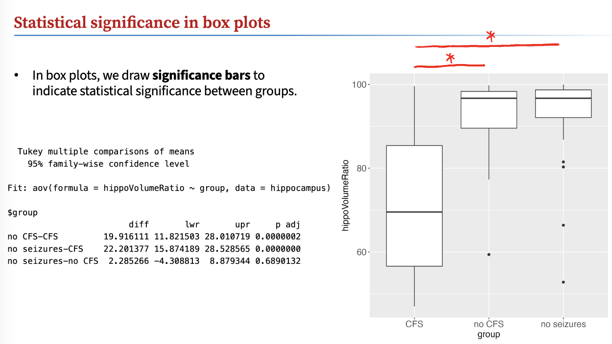
Tukey’s post-hoc Test and Interpretation

Post-hoc test: statistical test performed after initial test (ie, ANOVA) to find which pairs of groups are significantly different

Tukey’s post-hoc test: most common after ANOVA, if you reject the null

• first, run ANOVA; if reject null:

• run post-hoc test

  • TukeyHSD(result)

  • HSD stands for honestly significant difference

If p-value between groups are < 0.05, there is a significant difference!

• draw significance bars to indicate statistical significance between groups

Verifying normality in ANOVA

For ANOVA, we try to verify the data meet the assumptions using AS FEW TESTS as needed

• within each group, determine the residuals

  • Residuals: difference between each data point and its group mean

  • analyzing residuals can show non-normality

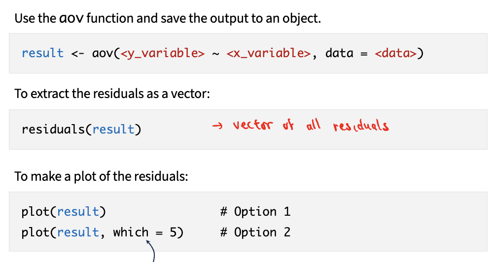
Steps:

• 1) use aov function and save output to object

• 2) extract residuals as vector

• 3) make plot of residuals

Non-parametric tests

Sometimes, your data may never meet the assumptions of a t-test/ANOVA (parametric test) regardless of transforming

• can use non-parametric tests, which do not assume normality

  • tests other attributes of data, ie median, rank order

  • generally have lower power

Paired t-test → Wilcoxon signed rank test

2-sample t-test → Mann-Whitney U test

ANOVA with Tukey’s post-hoc test → Kruskal-Wallis test with Dunn’s post-hoc test

Covariance

After finding (x - mean) (y - mean) for every data point, we calculate average

• more points in positive quadrants, positive covariance = positive association

• more points in negative quadrants, negative covariance = negative association

• equally many points in both positive and negative quadrants = zero association

Only sign of covariance is meaningful:

• same data, different units → different covariance

• covariance changes even though underlying relationship between variables did not change

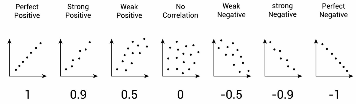
Pearson correlation coefficient

Normalize covariance by using r, called Pearson correlation coefficient

• is not sensitive to units

• r tells us if two variables rise and/or fall together

Does NOT imply a causal relationship between two variables!

• r only tells us whether two variables rise and/or fall together

Correlation vs Regression

Correlation: goal is to quantify the association between two numerical variables

• NOT trying to fit a line to the data

• JUST seeing if two variables rise/fall together

Regression: goal is to predict the value of one variable from another

• clearly defined independent and dependent variable

• we ARE trying to fit a straight line to the data

Linear model/regression model

Goal: predict the dependent variable from the independent variable

• draws straight line through the data, creates equation y = mx + b

Sample statistics (b1 and b0): estimate the population parameters (ß1 and ß0)

class 20

Least Squares Approach

Residual: difference between each y-value and model’s prediction

• across all data points, calculate sum of squared residuals

• better the model fits our data, the smaller the sum of squared residuals

  • y-value should be closer to model’s prediction

Best fit line (aka regression line): one that minimizes sum of squared residuals

• say this line was obtained using the “least squares approach”

Slope of the regression line

Slope is the biology!

• ex. plant mass = 0.92 x nitrogen levels + 10.7

• for every 1 ppm increase in nitrogen, plant mass increases by 0.92g

Y-intercept has no biological significance

• you should avoid extrapolating too far beyond the data

The better our model, the lower SS(model) is compared to SS(mean)

• SS measures error of the model

• Lower SS(model) → our model’s predictions are closer to the actual data

class 20

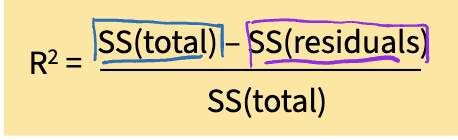
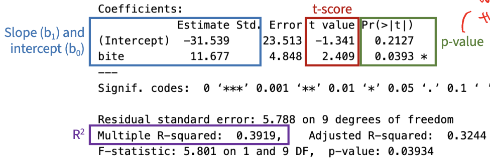
R² and its meaning

R²: proportion of the total variance of y that is explained by x

The sum of square went down from 16.05 → 8.58, 47% decrease!

• there is a 47% decrease in error when we take nitrogen levels into account

• 47% of the total variance in plant mass is explained by the soil nitrogen content

SS(mean) is often called SS(total)

• represents the total variability in the y variable

SS(model) is often called SS(residuals)

• represents the residuals of the final model

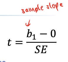
Null distribution of b1 values + comparing t-score with the null

theoretical distribution of all possible b1 values IF THE NULL IS TRUE

• due to random sampling, even when the null is true, the slope of our sample (b1) won’t be exactly zero

• the larger the magnitude of the t-score, the more likely we are to reject the null

Comparing our t-score with the null

• if null is true, we expect the t-score to be close to zero

• p-value: probability of getting OUR slope / OUR t-score or a more extreme value of the null is true

• if p < alpha, REJECT the null

Interpreting linear regression in R

Only care about the slope!

Since p-value of bite slope (11.677) is 0.0393:

• We reject the null, there is a relationship that exists between the variables

• IF THE NULL WERE TRUE, we have a 0.039 chance of getting a t-score (or a slope) as extreme as ours

• p < alpha

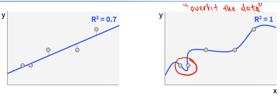
Overfitting

when model tries TOO hard to match the data

• even if the model perfectly describes the data we have, it will perform poorly on new, unseen data

• we never expect R² to be 1

• if you draw a squiggly line, unlikely that it is the true relationship

Comparing Residuals

Residuals: difference between each measurement and model

• when relationship is truly linear, some points are above and some are below the regression line

  • there is no pattern to the residuals; are normally distributed

• when relationship is non-linear, there is a pattern to the residuals

  • residuals are NOT normal

Transforming residuals for regression

1) Plot the residuals and run a KS test on the residuals

• if normal, linear regression is valid

• if non-normal:

2) make a histogram of the x and y variables

• is one variable clearly skewed?

• is one variable mostly normal but has a clear outlier?

  • transform skewed variable or remove the outlier

3) run a KS test on the new model residuals

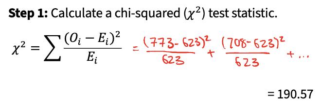
Chi-squared goodness-of-fit test

Used to perform hypothesis tests on categorical data:

Step 1: calculate a chi-squared (x²) test statistic

Step 2: predict the null distribution of x²

Step 3: compare our value of x² to the null distribution

Basically, compare observed frequency of category to expected frequency of category

Statistical Tests Summary

One sample t-test: 1 numerical

Paired t-test: two categories; 1 numerical, 1 categorical

Two-sample t-test: two categories; 1 numerical, 1 categorical

ANOVA: 3+ categories; 1 numerical, 1 categorical

Linear regression: 2 numerical

Chi-squared goodness of fit: 1 categorical

Correlation is also appropriate for quantifying association – it does NOT attempt to predict Y from X

Manipulative vs Natural Experiments

Manipulative: experimenter actively controls the independent variable

• more directly establish causality between independent and dependent variabels

• however, might not be practically and/or ethically feasible

Natural/Observational: experimenter relies on pre-existing differences in independent variable

• challenging to implement control group, randomly assigning subjects to treatment vs control groups, and blinding

Random vs Systematic Error

Random: fluctuations in our data that occur just by chance

• ie natural variation in blood pressure between individuals

Systematic: error that consistently skews our data in one direction

• ie meditation group starts to eat more healthily and exercise more

• includes confounding variables, non-random assignment, experimental bias

Minimizing systematic error

Control groups: isolate the effect of the treatment (IV) on DV

• to minimize confounding variables, keep control group maximally similar to treatment group

Random assignment: each experimental subject should have equal chance of being assigned to treatment or control group

Blinding: if participants or researcher are aware of treatment, may consciously or subconsciously influence their behavior

• Single-blind: participants unaware if they have been assigned to treatment or control

• Double-blind: BOTH participants AND researchers are unaware who is assigned to treatment or control

Sample Size and Random Error

If we only give each cream to one person, exposes us to LOTS of random error

• any observed difference could be significantly affected by natural variability between the two people

When you increase sample size, you give the skin creams to more people

• increasing sample size reduces the influence of random error

  • averages out random variation across more people

• any one individual now exerts a weaker pull on the overall mean

When increasing sample size, standard error of the mean decreases!

• smaller n → larger SE

• larger n → smaller SE

  • standard error is a measure of the random error!

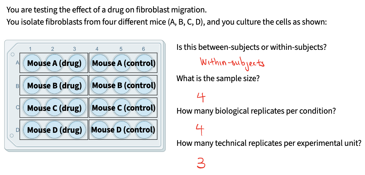
Experimental Unit + Between-subjects vs. within-subjects

An individual or group that is assigned a treatment independently of every other unit

• Between-subjects / between-groups: each experimental unit experiences EITHER one condition OR the other

  • unpaired

  • independent groups design

• Within-subjects / within-groups: each experimental unit experiences BOTH conditions

  • paired

  • repeated measures design

Sample size and replicates (biological vs technical)

Sample Size: total number of experimental units across entire experiment

Biological replicates: number of experimental units that experience each condition

• captures biological variability

Technical replicates: number of measurements you take per experimental unit

• increases precision of measurement

• does NOT capture any additional biological variation

Pseudoreplication and how to avoid it

Pseudoreplication: when you erroneously report the sample size as being higher than it actually is

• ex. if you take 4 measurements per plant, you think sample size = 6 plants x 4 measurements = 24

  • not correct! 4 measurements are technical replicates

To avoid pseudoreplication:

• Ask yourself: how do I increase sample size?

  • add more plants!

    • adding more experimental units / biological replicates

  • DO NOT take more measurements from each plant!

    • adding more technical replicants!

• increasing sample size = capturing more biological variability

Measurement Validity

Does my experimental system actually address the research question that I’m asking?

To validate, you need additional control groups:

• Negative control: checks if experimental system can detect a lack of change when we expect it to

  • ie mice receive an injection of DMSO solvent WITHOUT a supplement

  • establish baseline comparison WITHOUT any treatment

• Positive control: checks if experimental system can detect a change when we expect it to

  • ie mice receive an injection of a supplement KNOWN to raise blood insulin levels

  • verifies our system CAN detect a postive result

For both positive and negative controls, we KNOW what to expect

• check experimental system is behaving as it should

Comparing positive and negative controls

If there is no difference between the positive and negative controls, this undermines the validity of our data.

• injection was faulty?

• technique for measuring insulin is broken or not sensitive enough?

• incorrect dosage – all supplements are delivered at too low a concentration?