Intro to Statistics Final Exam

Population

a collection of persons, things, or objects under study.

Sample

selecting a portion (or subset) of the larger portion

Parameter

A numerical characteristic of the whole population that can be estimated by a statistic.

Ex: we consider all math classes to be the population, so the average number of points earned per student over all math classes is a parameter.

Statistic

A number that represents a property of the sample.

Ex: if we consider one math class to be the sample of the population of all the math classes, then the average number of points earned by a student in that one math class at the end of the term is an example of a statistic.

Variable

usually letters x and y, is a characteristic or measurement that can be determined for each number of the population

Numerical variable: takes on a value with equal units such as weights in pounds and time in hours.

Categorical variable: place the person or thing into a category (ex: party affiliation, gender, gpa).

Data

the actual values of the variable

What are the levels of measurement?

Nominal: no numerical value or order (names, labels, categories)

Ordinal: usually no numerical value, but there is an order, however, the differences between the data are meaningless (small, medium, large)

Interval: data can be ordered, and differences are meaningful

Ratio: can be ordered, differences are meaningful, and zero corresponds to none of the values (0 is a measurement)

simple random sample

each sample of the sample size has an equal chance of being selected; simple random sample from the entire population

Stratified Sampling

Divide the entire population into distinct subgroups called strata. The strata are based on a specific characteristic such as age, income, education level, and so on. All members of a stratum share the specific characteristic. Draw random samples from each stratum.

Cluster Sampling

Divide the entire population into pre-existing segments or clusters. The clusters are often geographic. Make a random selection of clusters. Include every member of each selected cluster in the sample. Randomly select some cluster.

Systematic Sampling

randomly select a starting point and take every nth piece of data from a listing of the population

Multistage Sampling

Use a variety of sampling methods to create successively smaller groups at each stage. The final sample consists of clusters.

Convenience Sampling

Involves selecting participants who are readily available without any attempt to make the sample representative of a population.

Midpoint

A point that divides a segment into two congruent segments

lower boundary + upper boundary

__________________________________________________ = midpoint

2

Class Width

the distance between lower (or upper) limits of consecutive classes

largest data value - smallest data value

________________________________________________________ = class width

desired number of classes

Frequency Table

efficiently displays data. Organizes data into classes and list the number of data points in each class; classes with 0 occurrences are also listed

Class Limit

First find class width, then add that to the smallest data value, and keep adding it until you get to the highest data value. (ex: if the smallest data value is 36, and the class width is 13, then you would add 13 to 36, and the upper class limit for that bin would be 48, and the lower class limit for the next bin would be 49)

Class Boundaries

Take class limits and do -.5 for the lower class limit and +.5 for the upper limit

Frequency

the number of times a value of the data occurs

Cumulative frequency

frequency of a class with added frequencies of classes before that one. (ex: if bin 1's frequency is 3, and bin 2's frequency is 2, then bin 1's cumulative frequency 3 and bin 2's cumulative frequency would be 5 because you added it with bin 1's frequency, and then you would add bin 2's frequency with bin 3's)

Relative Frequency

the ratio (fraction or proportion) of the number of times a value of the data occurs in the set of all outcome to the total number of outcome. Divide each frequency by the total number of data in the sample. (if there is 20 students in a class and bin 1's frequency was 3, the its relative frequency would be 3/20 or .15)

cumulative relative frequency

the accumulation of the previous relative frequencies, add all the previous relative frequencies to the relative frequency for the current row.

cumulative

__________________ = cumulative relative frequency

total

If bin 1's relative frequency was .15, and bin 2's relative frequency was .25, then bin 2's cumulative relative frequency is .40. Then that would be added to bin 3's relative frequency.

Normal Distribution

A continuous ransom variable (RV) with pdf

Standard Normal Distribution

a continuous random variable (RV) X ~ N(0, 1); when X follows the standard normal distribution, it is often noted as Z ~ N(0, 1).

z-score

a measure of how many standard deviations you are away from the norm (average or mean)

x - µ

z = ______________

σ

Central Limit Theorem

If x is a random variable that is normally distributed, then x̄ is normally distributed with the same mean and standard deviation of σ/srt n

µx̄ = µx σx̄ = σx/srt n

Law of Large Numbers

says that if you take samples of larger and larger size from any population, then the mean x̄ of the sample tends to get closer and closer to µ. For CCL, the larger n gets, the smaller the standard deviation gets

Mean

The average of scores that all have the same weight add all then divide by total number of scores

Weighted Mean

each score has a weight or frequency

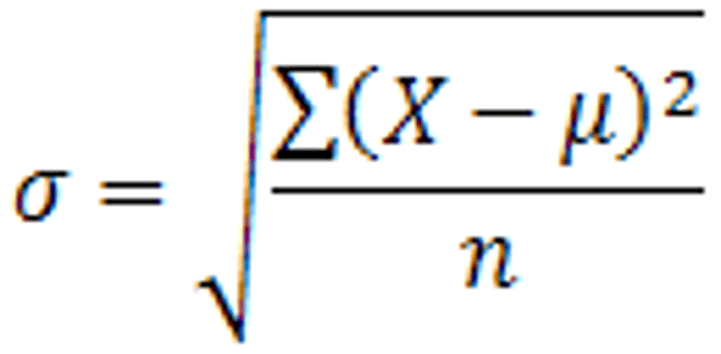
Standard Deviation

provides a numerical measure of the overall amount of variation in a data set and can be used to determine whether a particular data value is close to or far from the mean

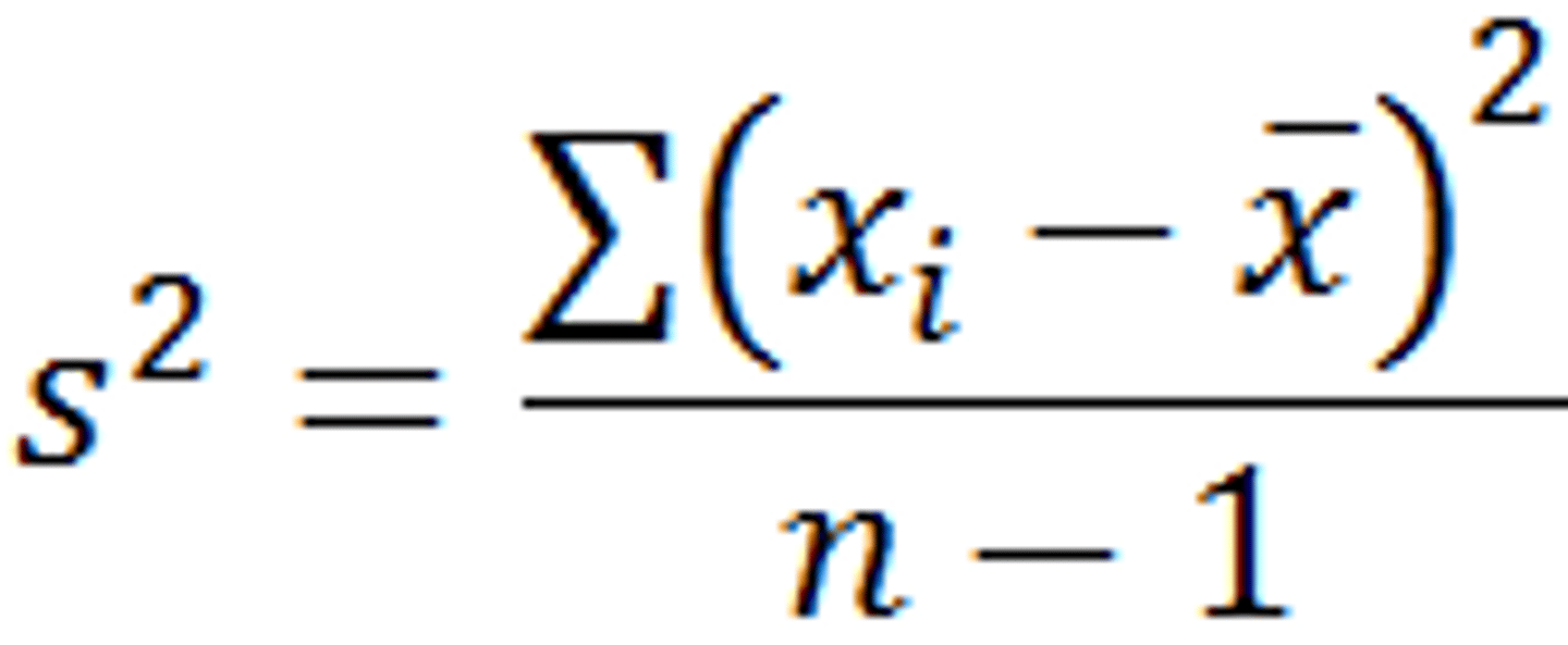
Variance

weighted average of squared deviation about the mean

Chebyshev's Inequality

Let x be a random variable having finite mean µ and finite variance σ^2. Let k be a strictly positive real number, then

P(|x - µ| < σ) >- 1 - 1/k^2

At least (1 - 1/k^2) of all the data in ANY data set/distribution falls with k standard deviation from the mean: x̄ - ks, x̄ + ks)

Discrete Probability Distribution

Listing of all the elements in the sample space and assigning a probability to every element

Expected Value

The mean of a probability distribution.

µ = sumof(x) = sumofx * p(x)

Binomial Experiment

- There are a fixed number of trials, n

- Each trial is independent, and each trial is repeated using identical conditions

- There are only two possible outcomes, called "success and "failure" for each trial

- The goal is to count the number of successes r in n trials

Binomial Probability Distribution

The random variable x = r is the number of successes obtained in the n independent trials.

Probability: P(x = r) = (n!/r!(n-r)!) * p^r (1-p)^n-r

Variance: Var(x) = σ^2 = npq

Mean: E[x] = µ = np

Standard deviation: σ = srt npq

The letter p denotes the probability of a success on one trial, and q denotes the probability of a failure on one trial. p*q = 1

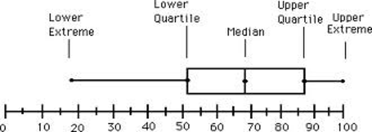
Box and Whisker Plot

provides a graphic display of the spread if the data about the median

Interquartile range = Q1 - Q3

Independent

If the knowledge that one occurred does not affect the chances of the other occurs

P(A|B) = P(A), P(B|A) = P(B) or P(A and B) = P(A)*P(B)

Dependent

If the two events are not independent

Mutually Exclusive

Events cannot occur at the same time. Meaning A and B do not share any outcomes and P(A and B) = 0

If it is not known whether it is mutually exclusive, assume they are not until you can show otherwise.

Multiplication Rule

Always involves the word AND

P(A and B) = P(B)*P(A|B)

or

P(A|B) = P(A and P)/P(B)

1. Independent (with replacement): P(A and B) = P(A)*P(B)

2. Dependent (without replacement): P(A and B) = P(A)*P(B|A)

Addition Rule

Always involves the word OR

1. Mutually Exclusive: P(A or B) = P(A) + P(B)

2. Not Mutually Exclusive:

P(A or B) = P(A) + P(B) - P(A and B)

^ must take out the overlap

When A and B are mutually exclusive, P(A and B) = 0

Null Hypothesis (Ho)

a statement of no difference between the variables - they are not related. This can often be considered the status quo and as a result if you cannot accept the null it requires some action.

Symbols:

Equal (=)

Greater than or equal to (≥)

Less than or equal to (≤)

Ho always has a symbol with an equal in it. The choice of the symbol depends on the wording of the hypothesis test

Alternative Hypothesis (Ha)

a claim about the population that is contradictory to Ho and what we conclude when we reject Ho. This is usually what the researcher is trying to prove.

Symbols:

Not equal (≠) or greater than (>) or less than (<)

Less than (<)

Greater than (>)

Ha never has a symbol with an equal in it. The choice of the symbol depends on the wording of the hypothesis test

Examples of Ho and Ha

Ho: No more than 30% of the registered voters in Santa Clara County voted in the primary election. p<-30

Ha: More than 30% of the registered voters in Santa Clara County voted in the primary election. p>30

We want to test whether the mean GPA of students in American colleges is different from 2.0 (out of 4.0)

Ho: µ = 2.0

Ha: µ ≠ 2.0

We want to test if college students take less than five years to graduate from college on the average.

Ho: µ ≥ 5

Ha: µ < 5

Possible Outcomes

all results that could occur from an experiment

____________________________________________________________________________

Action | Ho is | ....

______________________|_____________________________|_______________________

| True | False

______________________|_____________________________|_______________________

Do not reject | Correct Outcome | Type II error

Ho | |

______________________|_____________________________|_______________________

Reject Ho | Type I error | Correct Outcome | |

______________________|_____________________________|_______________________

What are the four outcomes in the possible outcomes table?

1. The decision is not to reject Ho when Ho is true (correct decision)

2. The decision is to reject Ho when Ho is true (type I error)

3. The decision is to not reject Ho when Ho is false (type II error)

4. The decision is to reject Ho when Ho is false (correct decision)

α

a.k.a sigma

α = probability of a Type I error = P(Type I error) = probability of rejecting the null when the null is true

should be as small as possible because it is the probability of error; they are rarely zero

β

a.k.a beta

β = probability of a Type II error = P(Type II error) = probability of not rejecting the null when the null is false

should be as small as possible because it is the probability of error; they are rarely zero

Distribution needed for Hypothesis Testing

Particular distributions are associated with hypothesis testing. perform tests of a population mean using a normal distribution or a student's t-distribution. (remember use a student's t-distribution when the population standard deviation is unknown and the distribution of the sample mean is approximately normal). We perform tests of a population proportion using a normal distribution (usually n is large).

To compare two means or two proportions, you work with two groups. The two groups are classified as:

Independent groups: consist of two samples that are independent, that is values selected from on population are not related in any way to sample values selected from the other population

- samples are independent

- test of two population means

- test of two population proportions

Matched pairs: consist of two samples that are dependent. The parameter tested using matched pairs is the population mean. The parameter tested using independent groups are either population means or population proportions

- samples are dependent

- test of the two population proportions by testing . one population mean of differences

The two independent samples are

simple random samples from two distinct populations.

for the two distinct populations:

- if the sample sizes are small, the distributions . are important (should be normal)

- if the sample sizes are large, the distributions . are not important (need not to be normal)

When conducting a hypothesis test that compares two independent population proportions, the following characteristics should be present:

1. The two independent samples are simple random samples that are independent

2. The number of successes is at least five, and the number of failures is at least five, for each of the samples

3. Growing literature states that the population must be at least 10 or 20 times the size of the sample. This keeps each population from being over-sampled and causing incorrect results

When using a hypothesis test for matched or paired samples, the following characteristics should be present:

1. Simple random sampling used

2. Sample sized are often small

3. Two measurements ((samples) are drawn from the same pair of individuals or objects

4. Differences are calculated from the matched or paired samples

5. The differences from the sample that is used for the hypothesis test

6. Either the matched pairs have differences is sufficiently large so that distribution of the sample mean of differences is approximately normal.

Decision and Conclusion:

A systematic way to make a decision of whether to reject or not reject the null hypothesis is to compare the p-value and a significance level:

- If α > p-value, reject Ho. The result of the sample data are significant. There is sufficient evidence to conclude that Ho is an incorrect belief and that the alternative hypothesis, Ha, may be correct.

- If α ≤ p-value, do not reject Ho. The results of the sample data are not significant. There is not sufficient evidence to conclude that the alternative hypothesis, Ha, may be correct.

- When you "do not reject Ho", it does not mean that you should believe that Ho is true. It simply means that the sample data have failed to provide sufficient evidence to cost serious doubt about the truthfulness of Ho.

If the p-value is low, the null must go

If the p-value is high, the null must fly

α > p-value => reject Ho

α ≤ p-value => fail to reject Ho

Assumptions for a hypothesis test of a single population mean µ using a Student's t-distribution (t-test):

- data should be a simple random sample that comes from a population that is approximately normally distributed

-use the sample standard deviation

1. the values in the sample must consist of independent observations

2. the population sampled must be normal

-used when we don't know the population standard deviation

-shorter middle and thicker tails than the standard normal distribution

-approaches standard normal for large degrees of freedom (df = n - 1)

Assumptions for a hypothesis test of a single population mean µ using a normal distribution (z-test):

- take a simple random sample from the population

- the population is normally distributed or your sample size is sufficiently large

- the value of the population standard deviation is known, which is rare

Assumptions for a hypothesis test of a single population proportion p:

- take a simple random sample from the population

- must meet the conditions for a binomial distribution, which are:

+ there are a certain number n of independent trials

+ the outcomes of any trial are success or failure

+ each trial has the same probability of a success p

- the shape of the binomial distribution needs to be similar to the shape of the normal distribution, to ensure this, the quantities np and nq must both be greater than 5 (np > 5 and nq >5). Then the binomial distribution of a sample (estimated) proportion can be approximated by the normal distribution with µ = p and σ = srt pq/n

*remember that q = 1-p

How to use the sample to test the null hypothesis

Use the sample data to calculate the actual probability of getting the test result, called the p-value. The p-value is the probability that, if the null is true, the results from another randomly selected sample will be as extreme or more extreme as the results obtained from the given sample.

A large p-value calculated from the data indicates we should not reject the null. The smaller p-value (more unlikely) the stronger the evidence is against the null. If the evidence is strongly against the null, we reject it.

Assumptions for ANOVA

-independence assumption

-equal variance assumption

-Normal population assumption

Chi-Square Distribution

A skewed distribution whose shape depends solely on the number of degrees of freedom. As the number of degrees of freedom increases, the chi-square distribution becomes more symmetrical.

χ ~ χ2df

df = degrees of freedom (dependent on how chi-square is used)

For the χ2 distribution, the population mean is µ = df and the population standard deviation is σ = srt 2(df)

The random variable is shown as χ2, but may be any uppercase letter

The random variable for a chi-square distribution with k degrees of freedom is the sum of k independent, squared standard normal variables. χ2 = (z1)^2 + (z2)^2 + .... + (zk)^2

1. the curve is non-symmetrical and skewed to the right

2. there is a different chi-square curve for each df

3. the test statistic for any test is always greater than or equal to zero

4. when df > 90, the chi-square curve approximates the normal distribution. For χ - χ2, the mean µ = df = 1,000 and the standard deviation, σ = srt 2(1,000) = 44.7. Therefore, χ ~ N(1,000, 44.7)

5. the mean, µ, is located just to the right of the peak.

To determine the "fit", you

use chi-square test ( meaning the distribution for the hypothesis test is chi-square). The null and alternative hypothesis for this test nay be written in sentences or may be stated as equations or inequalities. The test statistic for a goodness-of-fit is:

sumof(k) (O-E)^2/E

O = observed values (data)

E = expected values (from theory)

k = the number of different data cells or categories

The observed values are the data values and the expected values are the values you would expect to get if the null hypothesis were true. There are n terms of the form (O-E)^2/E

*The goodness-of-fit test is almost always right-tailed

test of independence

involve using a contingency table of observed (data) values.

the test statistic for a test of independence is similar to that of a goodness-of-fit test:

sumof(i*j) (O-E)^2/E

O = observed values

E = expected values

i = the number of rows in the table

j = the number of columns in the table

There are i*j terms of the form (O-E)^2/E

A tests of independence determines whether two factors are independent or not.

Test for Homogeneity

can be used to draw a conclusion about whether two populations have the same distribution. To calculate the test statistic for a test for homogeneity, follow the same procedure as with the test of independence

The expected value for each cell needs to be at least five (5) in order for you to use this test

Ho: the distributions of the two populations are the same

Ha: the distributions of the two populations are not the same

Test Statistic: uses a χ2 test statistic. It is computed in the same way as the test for independence

Degrees of Freedom (df): df = number of columns - 1

Requirements: all values in the table must be greater than or equal to five

Common Uses: comparing two populations. Ex: men vs. women, before vs. after, east vs. west. The variable is categorical with more than two possible response values.

Goodness-of-fit Test (chi-square)

use to decide whether a population with an unknown distribution "fits" a known distribution. In this case there will be a single qualitative survey question or a single outcome of an experiment from a single population. Tests to see if all outcomes occur with equal frequency, the population is normal, or the population is the same as another population with a known distribution. The null and alternative hypotheses are:

Ho: The population fits the given distribution

Ha: The population does not fit the given distribution

-test if data "fit" a particular distribution

-null and alternative hypothesis can be equations or written claims

-null hypothesis is always that the distribution "fits"

-is almost always a right-tailed test

Independence Test (chi-square)

use to decide whether two variables (factors) are independent or dependent. In this case there will be two qualitative survey questions or experiments and a contingency table will be constructed. The goal is to see if the two variables are unrelated (independent) or related (dependent). The null and alternative hypotheses are:

Ho: the two variables (factors) are independent

Ha: the two variables (factors) are independent

Homogeneity Tes (chi-square)

Use the test for homogeneity to decide if two populations with unknown distributions have the same distribution as each other. In this case there will be a single qualitative survey question or experiment given to two different populations. The null and alternative hypotheses are:

Ho: the two populations follow the same distributions

Ha: the two populations have different distributions

A test of a single variance

assumes that the underlying distribution is normal. The null and alternative hypotheses are states in terms of the population variance (or population standard deviation). The test statistic is:

(n-1)s^2/σ^2

n = the total number of data

s^2 = sample variance

σ^2 = population variance

The number of degrees of freedom is df = n - 1. A test of a single variance may be right-tailed, left-tailed, or two-tailed.

Linear Regression

for two variables, it is based on a linear equation with one independent variable. The equation has the form:

y = a + bx

where a and b are constant numbers. The variable x is the independent variable, and y is the dependent variable . Typically, you choose a value for the dependent variable.

The graph of the equation above is a straight line. Any line that is not vertical can be described by this equation.

For the linear equation y = a + bx

b = slope

a = y-intercept

The slope is a number that describes the steepness of a line, and the y-intercept is the y coordinate of the point (0, a) where the line crosses the y-axis.

Least Squares Criteria for Best Fit

The process of fitting the best-fit line is called linear regression. The idea behind finding the best-fit line is based on the assumption that the data are scattered about a straight line. The criteria for the best fit line is that the sum of the squared errors (SSE) is minimized, that is, made as small as possible. Any other line you might choose would have a higher SSE than the best fit line. The best fit line is called the least-squares regression line

Sample Space

The set of all outcomes of an experiment

Simple Event

A single element of the sample space (single element)

Event

any subset of the sample space (more than one element)

Notation

P(A): The probability of event A occurring

P(A^c): The probability of event A NOT occurring

number of outcomes in A

P(A) = _____________________________________________

Number of all possible outcome

Complement law: P(A^c) = 1 - P(A)

Conditional Probability

smaller subset of a sample space, where we know certain things must have happened

P(B|A) = the probability of B given A is known to have occurred

n(B and A)

P(B|A) =_____________________

n(A)

The numerator contains only those elements in both sets

The denominator contains only those elements in the "given" set

Properties of the Normal Distribution

unimodal, symmetric, approaching x-axis, and area under curve is 1

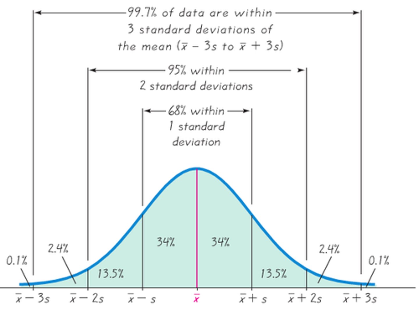
Empirical Rule

The rules gives the approximate % of observations w/in 1 standard deviation (68%), 2 standard deviations (95%) and 3 standard deviations (99.7%) of the mean when the histogram is well approx. by a normal curve

Confidence Intervals

the range on either side of an estimate that is likely to contain the true value for the whole population

will always have a special number attached called confidence level

Estimating Population Mean, µ

Requirements:

The random variable X has a normal distribution or n ≥ 30

c is the confidence level (0 < c < 1) and zc is the critical value for the confidence level based on the standard normal distribution

Estimating Population Proportion, p

Requirements:

np̂ > 5 and n(1-p̂) > 5

c is the confidence level (0 < c <1) and zc is the critical value for the confidence level based on the standard normal distribution.

*when preliminary value of p is not known, assume p̂ = 0.5

Estimating the Difference between population means, µ1 and µ2

Requirements:

The random variable X has a normal distribution or n ≥ 30

conclusions based on the confidence interval:

-if (+, +) -> (µ1 - µ2) > 0, then µ1 > µ2

-if (-, -) -> (µ1 - µ2) < 0 then µ1 < µ2

-if (-, +) -> (µ1 - µ2) could be positive or negative so we can't conclude a difference exists and the interval is inconclusive

Estimating the difference between proportions, p1 and p2

Requirements:

n1p̂ 1 > 5, n1(1 - p̂ 1) > 5

n2p̂ 2 > 5, n2(1 - p̂ 2) > 5

c is the confidence level (0 < c < 1) and xc is the critical value for the confidence level based on the standard normal distribution

Conclusions based on the confidence interval:

-if (+, +) -> (p1 - p2) > 0, then p1 > p2

-if (-, -) -> (p1 - p2) < 0, then p1 < p2

-if (-, +) -> (p1 - p2) could be positive or negative so we can't conclude a difference exists and the interval is inconclusive

Conducting a Hypothesis Test

1. Determine Ho and Ha, remember, they are contradictory

2. Determine the random variable

3. Determine the distribution for the test

4. Draw a graph, calculate the statistic, and use the test statistic to calculate the p-value ( a z-score and t-score are examples of test statistic)

5. Compare the preconceived α with the p-value, make a decision (reject or fail to reject the null), and write a clear conclusion in words and in terms of the alternative hypothesis.

Testing the Mean

if p < α, reject Ho and conclude Ha

if p ≥ α, fail to reject Ho and cannot conclude Ha

We "reject the null hypothesis and conclude the alternative at a significant level of α" or we "fail to reject the null hypothesis and cannot conclude the alternative at a significance level of α"

For two-tailed tests:

if the test statistic is on one side, double the area past it to calculate the p-value

Analysis of Variance (ANOVA)

ANOVA Assumptions:

-the population from which samples are drawn are normal

-samples are selected at random and are independent

-the populations are assumed to have equal variances

-the null hypothesis is that all the means are equal

-the distribution used for the test is the F distribution

-the F Ratio or F Statistic measures the variance between groups/variance within groups

-Hypothesis and Test

if p-value < α value, reject the null