MAC Module 16 The Short-Run Policy Trade-Off

The Phillips curve is useful for two reasons.

First, it focuses directly on two policy targets: the inflation rate and the unemployment rate. Second, the aggregate supply curve shifts whenever the money wage rate or potential GDP changes. 

The short-run Phillips curve shifts only when

the natural unemployment rate changes or when the expected inflation rate changes.

If the natural unemployment rate changes, both the

long-run Phillips curve and the short-run Phillips curve shift.

When the natural unemployment rate increases

both the long-run Phillips curve and the short-run Phillips curve shift rightward

when the natural unemployment rate decreases

 both the long-run Phillips curve and the short-run Phillips curve shift leftward.

The factors that influence the natural unemployment rate Those factors divide into two groups:

influences on job search and influences on job rationing.

The short-run Phillips curve

the downward-sloping relationship between the inflation rate and the unemployment rate when all other influences on these two variables remain the same.

 The short-run Phillips curve presents

a tradeoff between inflation and unemployment.

The short-run Phillips curve is another way of looking

 at the aggregate supply curve.

The long-run Phillips curve shows the relationship between

inflation and unemployment when the unemployment rate equals the natural unemployment rate and the inflation rate equals the expected inflation rate.

The long-run Phillips curve is

vertical at the natural unemployment rate, and there is no long-run tradeoff between unemployment and inflation.

When the expected inflation rate changes

the short-run Phillips curve shifts to intersect the long-run Phillips curve at the new expected inflation rate.

When the money growth rate changes,

the unemployment rate changes temporarily and eventually returns to the natural unemployment rate— the natural rate hypothesis.

A change in the natural unemployment rate shifts both

the SRPC and the LRPC curves.

The rational expectation of the inflation rate is based on

forecasts of the Fed’s monetary policy and its influence on aggregate demand growth.

A fall in the expected inflation rate improves

the short-run tradeoff.

Targeting the unemployment rate can only bring

temporarily lower unemployment and at the cost of permanently higher inflation.

The Phillips curve gets its name because

New Zealand economist A.W. (Bill) Phillips discovered it in 100 years of data on wage inflation and unemployment in the United Kingdom.

Short-Run Phillips Curve: The relationship was later found in the U.S. data and

in the data for many other economies.

The AS-AD model explains

the negative relationship between unemployment and inflation along the short run Phillips curve.

A movement along the AS curve is

equivalent to a movement along the short-run Phillips curve.

At the natural unemployment rate,

real GDP = potential GDP

When the unemployment rate is less than the unemployment rate,

real GDP exceeds potential GDP.

And when the unemployment rate exceeds the natural unemployment rate,

real GDP is less than potential GDP.

Okun’s Law

The relationship between the unemployment rate and real GDP.

Arthur Okun

an economic advisor to President John F. Kennedy, first observed the quantitative link between the unemployment rate and real GDP.

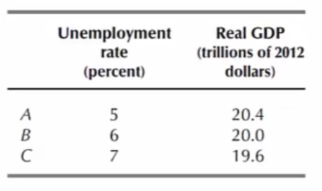
The table shows Okun’s Law. For each % point that the unemployment rate us above the natural unemployment rate

real GDP is 2% below potential GDP.

The inflation rate is defined

as the percentage change in the price level.

So starting any given price level,

the higher is the current period’s price level.

long-run Phillips curve

the relationship between inflation and unemployment when the economy is at full employment.

At full employment, the growth rate of the quantity of money determines the

inflation rate and any inflation rate is possible.

Natural rate hypothesis

the proposition that when the inflation rate changes, the unemployment rate changes temporarily and eventually returns to the natural unemployment rate.

If the natural unemployment rate changes,

both the long-run Phillips curve and the short-run Phillips curve shift.

When the natural unemployment rate increases,

both the long-run Phillips curve and the short-run Phillips curve shift rightward.

When the natural unemployment rate decreases,

both the long-run Phillips curve and the short-run Phillips curve shift leftward.

Changes in the natural unemployment rate have

changed the tradeoff.

According to the Congressional Budget Office, the natural unemployment rate increased from about

5 % in 1950 to more than 6 percent in the mid-1970s. It decreased to 5% by 2000 and then increased again to 5.5 percent by 2011, where it remains today.

The expected inflation rate is

the inflation rate that people forecast and use to set the money rage rate and other money prices.

A rational expectation is a forecast that uses all the

relevant data and economic science.

Suppose that the Fed wants to lower the

unemployment rate.

The Fed speeds up the growth rate of aggregate demand by

speeding up the growth rate of money and lowering the interest rate.

With a given expected inflation rate,

the unemployment rate initially falls and the inflation rate rises.

But if the Fed drives the unemployment rate below the natural rate

the inflation rate will continue to rise.

As the higher inflation rate becomes expected,

wages and prices start to rise more rapidly.

If the Fed keeps increasing aggregate demand,

the expected inflation rate rises.

Eventually, both inflation and unemployment will increase and

the economy will return to full employment and the natural unemployment rate.

If the Fed wants to lower the inflation rate, it can pursue two alternative lines of attack:

A surprise inflation reduction

A credible announced inflation reduction

This credible announced inflation reduction lowers the inflation rate but

with no accompanying loss of output or increase in unemployment.

In 1981, when we last faced a high inflation rate,

the Fed slowed it, & we paid a high price.

The Fed’s policy action was

unexpected so the unemployment rate went above the natural rate.

It was to 10 % for 2 years and

remained above the natural rate for 5 years.

The short-run Phillips curve is a curve that shows the relationship between the _____ rate and _____ when _____ and the _____ remain constant. 

A. inflation; the unemployment rate; the natural unemployment rate; expected inflation rate 

The long-run Phillips curve is the relationship between _____ and _____ when the economy is at full employment. The long-run Phillips curve is a _____ line at the _____ unemployment rate.

D. inflation; unemployment; vertical; natural

The expected inflation rate is the inflation rate that people forecast and use to set the _____ and _____. 

C. money wage rate; other money prices

The natural rate hypothesis is the proposition that when the _____ rate changes, _____ changes temporarily and eventually returns to _____. 

C. inflation; the unemployment rate; the natural unemployment rate

A rational expectation is a forecast that results from the use of all the relevant data and _____.

C. economic science 

The short-run Phillips curve shows that, other things remaining the same, ________.

D. a rise in the inflation rate and a fall in the unemployment rate occur together

The long-run Phillips curve ________.

B. is a vertical curve at the natural unemployment rate

The short-run Phillips curve intersects the long-run Phillips curve at ________.

C. the expected inflation rate and the natural unemployment rate

An increase in the expected inflation rate, other things remaining the same, ________.

A. shifts the short-run Phillips curve upward

​A ​decrease in the natural unemployment rate ________.

A. shifts both the short-run and the long-run Phillips curves leftward

Suppose that the unemployment rate exceeds the natural unemployment rate and the Fed increases the money growth rate. If the Fed’s action is ________.

A. unexpected, the unemployment rate falls but the inflation rate rises

Fluegges Lecture: Between the 1940s and 1970s, the Keynesians ruled the day, and Keynesian economists,

such as Paul Samuelson and Robert Solow, ruled policy debates.

 Fluegges Lecture: Milton Friedman was an early decenter from the Keynesian view, and

he with a leading group of macroeconomists, countered against against Keynes and fiscal policy. 

Fluegges Lecture: Friedman promoted monetary policy

as the more effective.

Fluegges Lecture:

While strict monetarism was short lived,

its effect brought into question the long-held stable policy prediction between inflation and unemployment, also known as the Phillips Curve

Fluegges Lecture: In the mid-1980s, the Keynesians and Classicals split

into their own schools, and there has been a greater synthesis between the two school's views. 

Fluegges Lecture: Although it still exists, the most current rendition of this policy dichotomy

is rules versus discretion.

Scotts Lecture: 1936 Keynes

1- Markets inefficient

2- Gov’t active

3- Unemployment is involuntary

Scotts Lecture: 1968 - Milton Friedman

Deactivist policy detrimental ↓

Scotts Lecture: 1985 -

PAyrn insight

Scotts Lecture: Activist policy

Gov’t has an active role to control business

Scotts Lecture: Markets are

efficient

Scotts Lecture: Debt is

all of the debt

Scotts Lecture: Deficit is

the debt of each year

Scotts Lecture: Structural deficit/ Deficit Debt /

GDP

Scotts Lecture: Wealth = accumulation

Adam Smith 1759 Theory of Moral Sentimentals, 1776 Wealth of Nation

Scotts Lecture: Wealth = production

A - Specialize

B- Trade Classicals

Scotts Lecture: A.S. Ricardo Malthus, Marx TS Mill

1- Markets, efficient

2- Gov’t limited role

Scotts Lecture:

Austerity results

There is no question regarding the non-linear result.

At some point, a country’s debt burden eventually hurts its ability to borrow.

Scotts Lecture:

Austerity results

The threshold is debatable,

and different size economies have varying abilities to carry debt.

Scotts Lecture:

Austerity results

Keynesian economists

mock austerity.

Scotts Lecture:

Austerity results

Classical economists

remain cautious.

Scotts Lecture:

This Time is Different: Considers international financial crisis history

1. Two types of debt defaults: explicit and implicit.

2. Non-linear relationship between a country’s ability to carry debt and when the size of their debt becomes a burden

3. Why this time is never different.

Scotts Lecture: Austerity measures are often used by governments

that find it difficult to borrow or meet their existing obligations to pay back loans.

Scotts Lecture: Economic Austerity

a set of economic policy principles that aim to reduce the government budget deficits through of both. Austerity’s primary objectives is to reduce a country’s structural deficit so that international debt markers continue to lend a country.

Scotts Lecture: There are 3 primary types of austerity measures:

1. higher taxes to fund spending

2. raising taxes while cutting spending

3. and lower taxes and lower government spending event more

Scotts Lecture: Crowding out

Scotts Lecture:

Myth: If we keep offering debts, our country will go bankrupt.

Reality: The government debt is an obligation to pay U.S. dollars. If the government were in a pinch, it would simply print more U.S. dollars.

Scotts Lecture:

Myth: The government is like a household. If it spends more then it collects, it must sell assets to pay its debt.

Reality: Government is like a corporation. Corporations are a legally recognizable entity. As such, never dies. Since the corporation never dies, it can simply roll over its debts into future generations. Government also never dies and can pass on its debt to future generations.

Scotts Lecture:

Myth: It is immoral for government to carry a debt. How can it expect citizens to honor their debts if government is not willing to pay off its debt.

Reality:

Government debt $6 trillion

Corporate debt $12 trillion

Personal debt $16-18 trillion

Scotts Lecture: The debt is

the cumulative sum of annual deficits.

Scotts Lecture: We have has a positive debt since

Andrew Jacksons administration

Scotts Lecture: What causes a deficit?

1. → Automatic stabilizers

2. Wars

3. Social expenditures

   1. A - Social security

   2. B- Medicare

4. Tax cuts

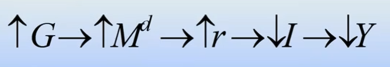
Scotts Lecture: Why borrowing is bad

Contraction: An increase in government expenditures was supposed to increase output. However, the increase crowded-out investment.

Scotts Lecture:

Deficit:

Government Expenditures- Taxes

Scotts Lecture: The amount that government expenditures exceed tax revenue.

However, government must still pay for its expenditures. To bridge the gap during a recession, government usually borrows money in the money market to cover its deficit.

Scotts Lecture: Government was in surplus the last year of

Clinton’s administration.

Scotts Lecture: Why printing is bad. Printing leads to too many dollars chasing few goods.

This leads to inflation.

• Makes contracts unstable.

• Redistribution of wealth

Scotts Lecture: During a contraction, raising taxes takes money-

out of consumers hands and further exasperates the contraction.