tamu Math 140 final

cost function

C(x)=mx+b

variable cost+fixed cost

revenue function

R(x)=p*x

profit function

P(x)= R(x)-C(x)

break even quantity

R(x)=C(x) (or P(x)=0)

where revenue and cost intersect

equilibrium point

S(x)=D(x)

where supply and demand intersect

how to determine which number to pivot

a) Find the MOST NEGATIVE element in the last row. This determines the pivot column. If there

are two that have the same most negative value, either one is fine.

(b) For each POSITIVE entry above the horizontal line in the pivot column, divide the constant on

the right side of the vertical line by the corresponding element in the pivot column. The row

with the smallest ratio becomes the pivot row. If there is a tie between smallest ratio, defalt goes to the one that's in the highest row.

(c) The element where the pivot column and row intersect is the pivot element.

how do you know when you're done pivoting

when there's no more negative numbers in the bottom row

elementary operations

yield an equivalent system of equations

•A matrix is in echelon form if:

1. The first nonzero element in any row is 1, called the leading one.

2. The column containing the leading one has all elements below the leading one equal to 0.

3. The leading one in any row is to the left of the leading one in a lower row.

4. Any row consisting of all zeros must be below any row with at least one nonzero element.

Gauss elimination

procedure for a systematically using elementary

operations to reduce a system of linear equations to an equivalent system whose solution set can be immediately determined by backward substitution.

order of a matrix

m × n where m is the number of

rows and n is the number of columns.

element in the ith row and jth column of a matrix A is denoted by

A(ij)

transpose of a matrix

represented by A^T

switch the rows and the columns

row matrix

matrix with one row

column matrix

matrix with one column

square matrix

matrix with equal number of rows and columns

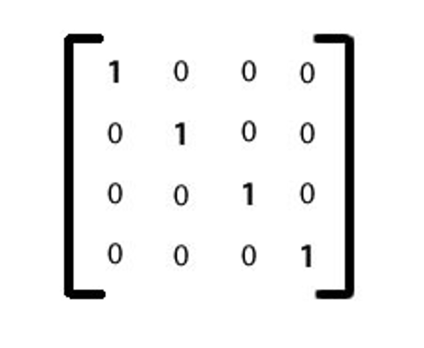
identity matrix

Matrix multiplication properties

A(BC) = (AB)C

A(B+C) = AB+AC

AIn= InA = A

(In is identity matrix)

A^-1(A)=In

objective function

subject to

the function we are maximizing or minimizing

subject to constraints in the form of inequalities

Steps to graphing an inequality.

1. Replace (temporarily) the inequality sign by an equal sign and graph the line. If the inequality is <

or >, use a dashed line. If the inequality is ≤ or ≥, use a solid line.

2. Shade the side of the line that satisfies the inequality, i.e. that makes the inequality true. Label the solution set/feasible region S.

corner points

-the points where the boundary line of the region changes

-easiest way to find points is to set the two lines equal to one another to solve where they intersect

Method of Corners

1. Graph the feasible region. Label it S.

2. Find the coordinates of all corner points.

3. Evaluate the objective function at each corner point.

4. Find the corner point(s) that gives the maximum or minimum value (if one exists).

(a) If there is only one vertex where the max/min is attained, this is the unique solution.

(b) If the objective function is optimized at two adjacent vertices of S, then it is optimized at EVERY point along the line segment connecting these two vertices. In this case, there are infinitely many solutions.

basic variable

column is one that consists of ones and zeroes only

non-basic variables

all other columns that contain more than ones and zeroes

• E^c

is the event that E does NOT occur.

E ∪ F

is the event that E OR F (or both) occur.

E ∩ F

the event that BOTH E AND F occur

Rules of Probability:

1. 0 ≤ P(E) ≤ 1 for any event E in a sample space S. In particular P(∅) = 0 and P(S) = 1.

2. Union rule for probability: If E and F are ANY two events, then P(E ∪ F) = P(E) + P(F) − P(E ∩ F)

Note: If E and F are mutually exclusive, then E ∩F = ∅, which means P(E ∩F) = 0 and the formula

reduces to just P(E ∪ F) = P(E) + P(F).

3. Complement Principle: P(E^c) = 1 − P(E) or P(E) = 1− P(E^c)

expected value of a random variable

E(X) = x1p1 + x2p2 + . . . + xnpn

when is a game considered fair

when the expected value equals zero

degree of the polynomial

highest power of x that appears.

leading coefficient

the coefficient of the highest power of x

zeros of a function

x-intercepts of the function

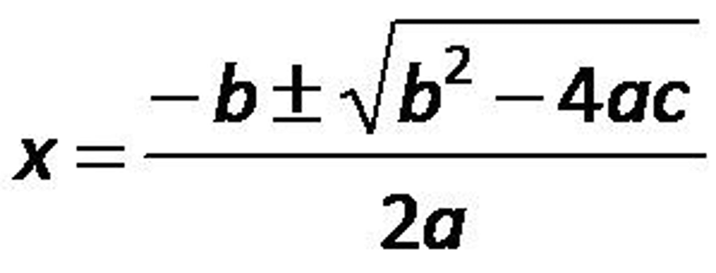
quadratic formula

vertex of a function

x=-b/2a

then plug into function to get y value

difference quotient

(f(x+h)-f(x))/h

domain rules for radical funtions

-if even root, anything under radical has to be set greater than or equal to zero

-if an even root is in the denominator than it should be set greater than zero

-it's fine if it's an odd root

-if odd root is in the denominator than it should be set greater than zero

how to rationalize a numerator or denominator

multiply it by its conjugate

exponent properties

1.)a^x=a^y then x=y

2.)a^0=1

3.)a^m*a^n=a^m+n

4.)a^m/a^n=a^m-n

5.)(a^m)^n=a^mn

6.)a^-n=1/a^n

7.)(ab)^n=a^n*b^n

8.)(a/b)^n=(a^n/b^n)

9.)a^(m/n)=n√a^m

exponential function

f(x)=a^x

where a is greater than 1

important exponential function

f(x)=e^x

e ≈ 2.71828

compound continuously

A(t) = P e^rt

logarithmic properties

loga(x)=b is equal to a^b=x

loga(xy)=loga(x)+loga(y)

loga(x/y)=loga(x)-loga(y)

loga(x^c)=cloga(x)

logarithm rules

you can't take the log of a zero or a negative number so set everything greater than zero

interest

accumulated amount

I=Prt

A=P+I

A=P+Prt

A=P(1+rt)

compound interest

F=P(1+r/m)^mt

we use TVM solver in calculator

effective interest rate

also done in calculator

eff(I,m) where I is the %interest/year, compounded m times a year

annuities

-when PMT not longer equals zero

-PMT will be made at the end of each period

*PMT and PV should be -, and FV should be +

sinking fund

-an account that is set up for a specific purpose at some future date

-ex: a family wants to save up a certain amount of money so find how much they should deposit each time to reach their goal

*PMT and PV should be -, and FV should be +

amortization

-when dealing with loans or mortgages

*PMT is -, and PV and FV should be +

Outstanding principal

-how much you still owe on the loan at a given point

-find the future value of the loan after the number of payments made up to that point

Equity

equity= total value of item-outstanding principal