CSCI 164 Midterm 1

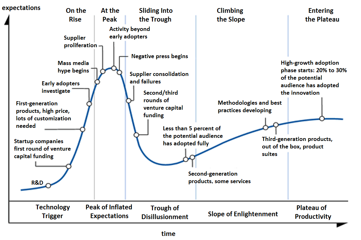
Gartner Hype Cycle

When new technologies make bold promises, how do you discern the hyper from what’s commercially viable? And when will such claims pay off, it at all?

Provides a graphic representation of the maturity and adoption of technologies and applications, and how they are potentially relevant to solving real business problems and exploiting new opportunities

Innovation Trigger

First Phase of Gartner Hype Cycle

A potential technology breakthrough kicks things off

Early proof of concept stories and media interest triggers significant publicity

Often no usable products exist, and commercial viability is unproven

Peak of Inflated Expectations

Second Phase of Gartner Hyper Cycle

Early publicity produces a number of success stories, often accompanied by scores of failures

Some companies take action; many do not

Trough of Disillusionment

Third Phase of Gartner Hype Cycle

Interest wanes as experiments and implementations fail to deliver

Producers of the technology shake out or fail

Investments continue only if the surviving providers improve their products to the satisfaction of early adopters

Slope of Enlightenment

Fourth Phase of Gartner Hype Cycle

More instances of how the technology can benefit the enterprise start to crystallize and become more widely understood

Second and third generation products appear from technology providers

More enterprises fund pilots, conservative companies remain cautious

Plateau of Productivity

Fifth and Final Phase of Gartner Hyper Cycle

Mainstream adoption starts to take off

Criteria for assessing provider viability are more clearly defined

The technology’s broad market applicability and relevance are clearly paying off

1950s-1960s

First AI Boom

“GOFA!”

The age of reasoning, prototype AI developed

1970s

AI Winter 1

1980s-1990s

Second AI Boom

“Expert Systems”

The age of knowledge representation (appearance of expert systems capable of reproducing human decision making)

1990s

AI Winter 2

2000s-2010s

Third AI Boom

Machine Learning

Deep learning, autonomous vehicles

Turing Test

Machines that think

* How to define thinking?
* Machine to carry a conversation

Does not directly test whether the computer behaves intelligently

Tests only whether the computers behaves like a human being.

Test can fail in accurately measure intelligence in 2 ways: Some human behavior is unintelligent, some intelligent behavior is inhuman

Failed to understand the need for knowledge, scalability, to have sensors for getting data

Subsymbolic AI

Model intelligence at a level similar to the neuron

Let such things as knowledge and planning emerge

Symbolic AI

Manipulation of symbols

Model such things as knowledge and planning in data structures that make sense to the programmers that build them

Based on high-level symbolic (human-readable) representations of problems, logic, and search

Uses tools such as logic programming, production rules, semantic nets and frames, and it developed application like knowledge based systems / expert systems, symbolic mathematics, automated theorem provers, ontologies, the semantic web, and automated planning and scheduling systems

Counter example

Deductive Reasoning

This type of legitimate data point that refutes a premise that otherwise has a lot of support

Example

* Premise: All primes are odd
* Support: There are infinite number of odd primes
* Counterexample: 2 is prime and is not odd

Outlier

Inductive Reasoning

A data point that represents an unusual event or errant reading, and it does not reflect the overall trends and/or statistics

Example

* Premise: We have a fair coin. There’s a 50/50 chance it comes up heads
* Data: A dozen different experimenters flip the coin 10 times each. The number of heads seen by each: 5, 6, 3, 5,6, 6, 4, 5, 4, 10, 5, 4
* Outlier: Most of the data is within 1 standard deviation of the mean. The 10, however, is more than standard deviations from the mean. This can happen due to random variation, but not very often. Suggests this.

Graphs

Widely used in AI

* To model how different objects are connected
* To model a sequence of actions
* To define finite state machines
G = (V, E)
* V = Set of vertices
* E = Set of edges

Adjacency List

Data structure
Consists of an Array Adj or |V| lists
One list per vertex
For u ∈ V, Adj[u] consists of all vertices adjacent to u
If weighted arcs, then store weights as well
For directed graphs
- Sum of lengths of all is ∑ out-degree(v) \= |E|, number of edges leaving v
For undirected graphs
- Sum of lengths of all is ∑ degree(v) \= 2|E|

O(V + E)

Total storage of an Adjacency List

Advantages of Adjacency list

Space efficient, when a graph is sparse
Can be modified to support many graph types

Disadvantages of Adjacency List

Determining is an edge (u, v) ∈ G: not efficient
Have to search in u's adjacency list -\> O(degree(u)) time
O(V) in the worst case

Adjacency Matrix

Matrix A
- Size |V| x |V|
- Number vertices from 1 to |V| in some arbitrary manner
- A is defined by: A[i, j] \= a_ij \= 1 if (i, j) ∈ E, else 0

O(N^2)

Space of an adjacency matrix

O(1)

Edge insertion/deletion for an adjacency matrix

O(N)

Find all adjacent vertices to a vertex for an adjacency matrix

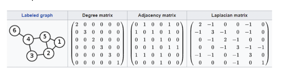
Degree Matrix

Consider a graph G \= (V, E) with |V| \= n
This is a diagonal matrix (size n x n) with d_ij \= Deg(v_ij) if i \= j, else 0
Special case: Directed graph -\> degree \= InDegree or OutDegree

Laplacian Matrix

Consider a graph G with n vertices
This is L_nxm is: L \= D-A
where D is the degree matrix, A is the adjacency matrix
- Simple graph -\> matrix contains only 0 and 1, diagonal \= 0
L_ij \= Deg(v_i) if (i \== j), -1 if i!\=j and v_i is adjacent to v_j, 0 otherwise

Incidence Matrix

A graph whose oriented incidence matrix M
Size |E|x|M| with element M_ev
- For edge e connecting vertex i and j, with i \> j and vertex v given by
M_ev \= 1 if v \== i
M_ev \= -1 if v \== j
M_ev \= 0 otherwise

Affinity Matrix

Also known as Similarity Matrix
An essential statistical technique used to organize the mutual similarities between a set of data points
Similarity is similar to distance but it does not satisfy the properties of a metric
- 2 points that are the same will have a similarity score of 1 while computing the metric will result in 0
- Similarity measure can be interpreted as the probability that 2 points are related
- If data points have coordinates that are close, then their similarity score will be much closer to 1 than 2 data points with a lot of space between them
Examples: Smart informational retrieval, advanced genetic research, efficient data mining, semi-supervised learning

Graphs in AI

G \= (V, E)
V: locations, positions in a map
E: roads, possible paths between locations
Weight of the edge (v_i, v_j):
- Cost to go from v_i to v_j: it can be the Euclidean distance
Applications: Video games, maps

Map

Graph of positions
Vertices: Cells on the map \= squares, hexagons
Edges: Connections to the cells in the neighborhood + special cases
Able to connect neighbors with Euclidean or Manhattan distance

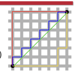
Manhattan Distance

A measure of travel through a grid system like navigating around the buildings and blocks of Manhattan, NYC.
D = |x1 - x2| + |y1 - y2|

Red, Yellow, Blue lines

Euclidean Distance

A method of distance measurement using the straight line mileage between two places. D = √((x2- x1)^2 + (y2 - y1)^2)

Green line

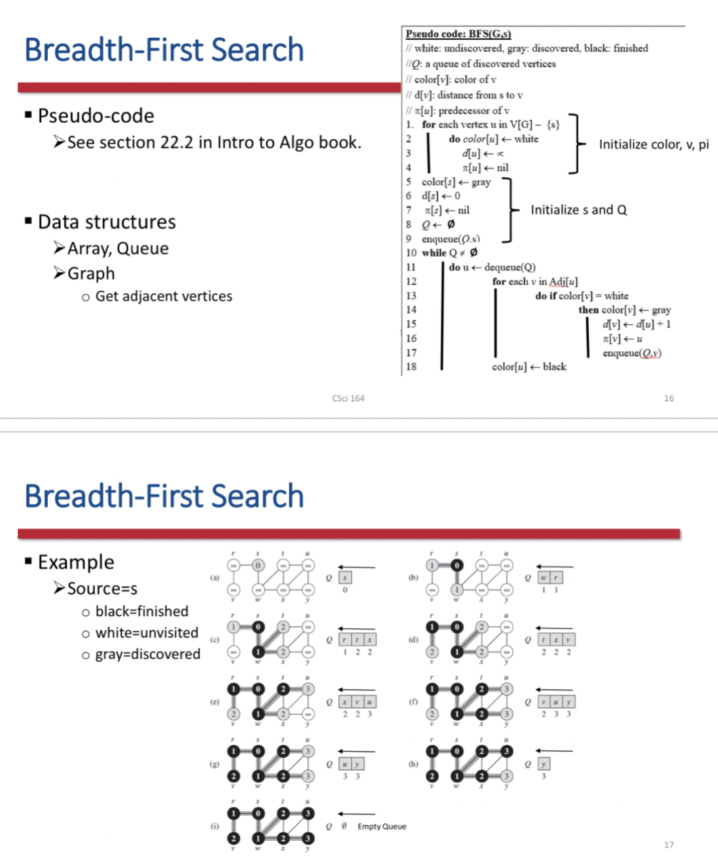
Breadth First Search

Algorithm for search a tree data structure for a node that satisfies a given property
- Starts a tree root (defined by the user) and explores all nodes at the present depth prior to moving on to the nodes and the next depth level
- Use a queue (FIFO) is needed to keep track of the child nodes that have been visited but not yet explored
Goal: Can be used to attempt to visit all nodes of a graph in a systematic manner
Input: Graph, directed or undirected, weighted or unweighted
Starts with a given node, then visits nodes adjacent in some specified order
Implementation
- Maintain an enqueued array
- Visit node after dequeued
- Then enqueue unenqueued nodes adjacent to the node

Use of BFS

AI Example: A chess game
1) A chess engine may build the game tree from the current position by applying all possible moves
2) Use a BFS to find a win position for white
- Implicit trees (like game trees or other problem solving trees) may be of infinite sizes
- BFS is guaranteed to find a solution node if it exists
Is a shortest path algorithm for unweighted graphs

O(V+E)

Initialization takes O(V)
Total time for queuing is O(V)
The sum of lengths of all adjacency lists is O(E)
Run time of BFS

Predecessor subgraph

For a graph G \= (V, E) with source s
This of G is G_𝜋 \= (V_𝜋, E_𝜋) where
V_𝜋 \= {v∈V: 𝜋[v] ≠ NIL|} ∪ {s}
E_𝜋 \= {(𝜋[v], v)∈E: v ∈ V_𝜋 - {s}}
Is a BF Tree is
- V_𝜋 consists of the vertices reachable from s
- ∀ v ∈ V, ∃! simple path from s to v in G_𝜋 that is also a shortest path from s to v in G
The edges in E_𝜋 are called Tree edges
- |E_𝜋| \= |V_𝜋| - 1

BFS Graph compression

Only 1 edge between a sequence of vertices
Detect hallways
Consider the type of connection between 2 vertices
- Mapping to the 2D or 3D environment
Isolate the key points, where the agents must go and potential intersections

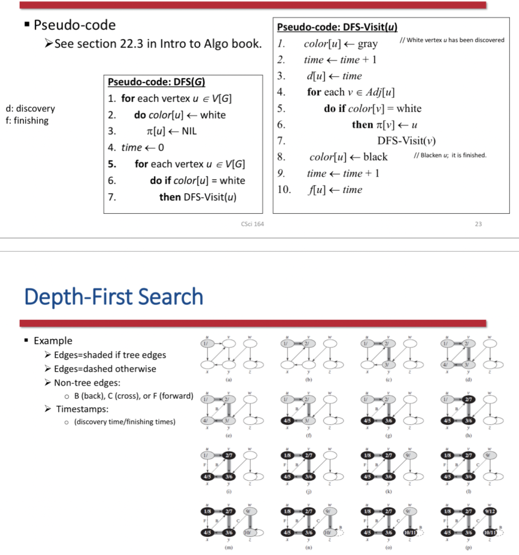
Depth First Search

Goal: To attempt to visit all nodes of a graph in a systematic manner
Input: Graph, directed or undirected, weighted or unweighted
Steps
- Explore edges out of the most recently discovered vertex v
- When all edges of v have been explored, back track to explore other edges leaving the vertex from which v was discovered (its predecessor)
- Search as deep as possible first
- Continue until all vertices reachable from the original source are discovered; If any undiscovered vertices remain, then one of them is chosen as a new source and search is repeated from that source

Shortest Paths

Problem: Find the sequence of vertices and edges in a graph G \= (V, E) from vertex start to vertex end
Rationale: To not test all possible paths
Property: A shortest path between 2 vertices contains other shortest paths within it

Weighted Directed Graph

G \= (V, E)
Weight function w: E -\> R (set of real numbers)
- Mapping of edges to real-valued weights
- w(p) of path \=

Single destination shortest path

Find a shortest path to a given destination vertex t from each vertex v
By reversing the direction of each edge in the graph, we can reduce this problem to a single-source problem

Single pair shortest path

Find a shortest path from u to v for given vertices u and v
If we solve the single source problem with source vertex u, this problem is also solved
All known algorithms for this problem have the same worst-case asymptotic running time as the best single source algorithms

All pairs shortest paths

Find a shortest path from u to v for every pair of vertices u and v
Although we can solve this problem by running a single source algorithm once from each vertex, we usually can solve it faster

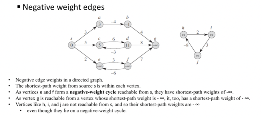
Special cases of shortest path

Cannot contain negative weight cycles
Cannot contain a positive weight cycle because removing the cycle from the path produces a path with the same source and destination vertices and a lower path weight

Representation of shortest paths

Let G \= (V, E)
- For each vertex v ∈ V a predecessor v.𝜋 (another vertex or NIL)
The shortest paths algorithms set the 𝜋 attributes so that the chain of predecessors origination at a vertex v runs backwards along a shortest path from s to v
Same as Breadth First Search
- predecessor subgraph G_𝜋 \= (V_𝜋, E_𝜋 induced by the values
- V_𝜋: the set of vertices of G_𝜋 with non NIL predecessors _ the source s
- V_𝜋 \= {v∈V: 𝜋[v] ≠ NIL|} ∪ {s}
- E_𝜋: the set of edges induced by the values for vertices
- E_𝜋 \= {(𝜋[v], v)∈E: v ∈ V_𝜋 - {s}}
Let G \= (V, E)
- A weighted, directed graph with weight function w: E -\> R
- AssumptionL G contains no negative weight cycles reachable from the source vertex s∈V (for well defined shortest paths)

Shortest Path tree

Same as BFS tree but contains shortest paths from the source defined in terms of edge weights instead of numbers of edges
A directed subgraph G \= (V', E') with V' ⊆ V and E' ⊆ E
- V' is the set of vertices reachable from S in G
- G' forms a rooted tree with root s
- For all v∈V' the unique simple path from s to v in G' is a shortest path from s to v in G

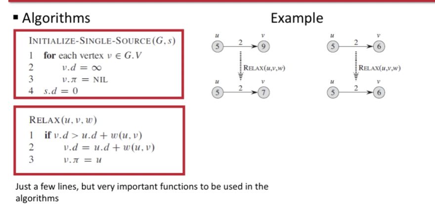
Relaxation

For each vertex v ∈ V we maintain an attribute v.d, an upper bound on the weight of the shortest path from source s to v
- v.d \= shortest-path estimate
Principle: Process of relaxing an edge (u, v) consists of testing whether we can improve the shortest path to v found so far by going through u and, if so, updating v.d and v.𝜋

Triangle Inequality

Relaxation Property
For any edge (u, v) ∈ E, we have 𝛿(u, v) ≤ 𝛿(s, u) + w(u, v)

Upper bound property

Relaxation property
We always have v.d ≤ 𝛿(s, v) for all vertices v ∈ V
Once v.d achieves the value 𝛿(s, v) it never changes

No path property

Relaxation Property
If there is no path from s to v, then we always have v.d \= 𝛿(s, v) \= infinity

Convergence Property

Relaxation Property
If s-\>u -\> v is a shortest path in G for some u, v ∈ V, and is u.d \= 𝛿(s, u) at anytime prior to relaxing edge (u, v) then v.d \= 𝛿(s, u) at all times afterward

Path relaxation property

Relaxation Property
If p \=

Predecessor Subgraph property

Once v.d \= 𝛿(s, v) for all v ∈V, the predecessor subgraph is a shortest paths tree rooted at s

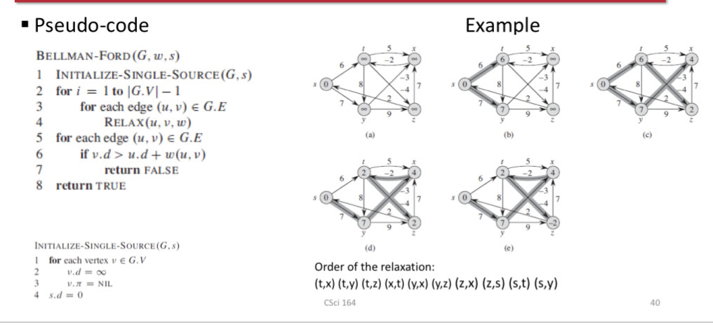
Bellman Ford Algorithm

Features
- Detects whether a negative weight cycle is reachable from the source
- Returns a Boolean value (true or false): whether or not there is a negative weight cycle that is reachable from the source
Principle: Relaxes edges, progressively decreasing an estimate v.d on the weight of a shortest path from the source s to each vertex v until it achieves the shortest path weight from s
Complexity: O(VE)

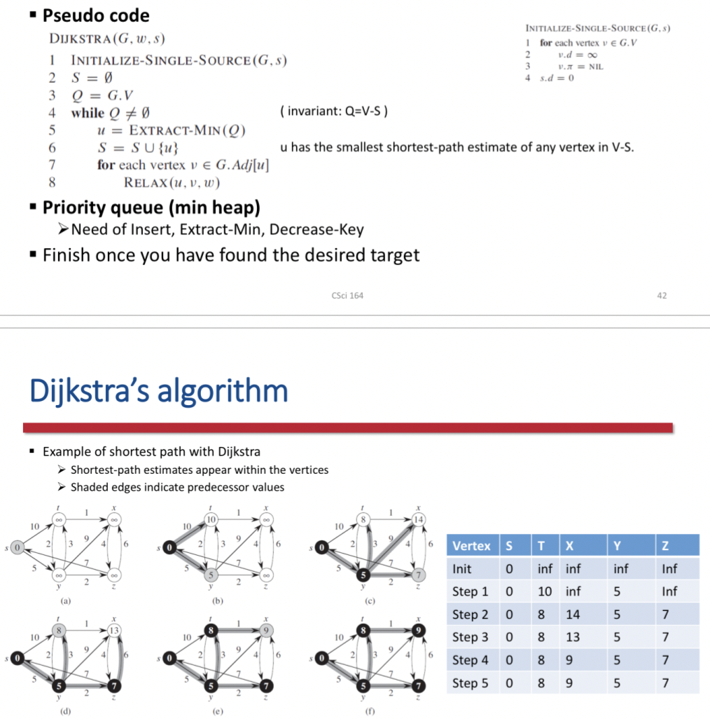
Dijkstra's Algorithm

Greedy algorithm
- Always choose the lightest or closest vertex in V-s to add to set S
- Does computer shortest path
Edge weights in the input graph are non negative
- w(u, v) \>\= 0 for each edge (u, v) ∈ E
Principle
- Repeatedly select the vertex u∈V-S with the minimum shortest-path estimate
- Adds u to S
- Relaxes all edges leaving u
Data structure: Min priority queue of vertices (Q)
- Vertex added/removed from Q: only 1 time
To show that it's correct
- u.d \= 𝛿(s, u) for all vertices u ∈ V

h(n)

Heuristic Function

Estimated cost of the cheapest path from the state at node n to a goal state

Heuristic

Technique designed for solving a problem more quickly when classic methods are too slow, or for finding an approximative solution when classic methods fail to find any exact solution

Goal: To obtain a good enough solution in a reasonable time frame

When to Use: Optimality, Completeness, Accuracy and precision, Execution time

Greedy best first search (GBF)

\n Goal is to expand the node that is closest to the goal , on the grounds that this is likely to lead to a solution quickly

Evaluates nodes by using just the heuristic function

f(n) = h(n)

A\* Search

Evaluates nodes by combining g(n), the cost to reach the node, and h(n) the cost to get from the node to the goal

f(n) = g(n) + h(n) = estimated cost of the cheapest solution through n

Both complete an optimal

Similar to Dijkstra's shortest path but add h(n) to the cost of the shortest path

Tree search version is optimal if h(n) is admissible

Graph search version is optimal if h(n) is consistent

Admissibility

Condition 1 for Optimality of A\* search

Never overestimates the cost to reach the goal

Optimistic because they think the cost of solving a problem is less than it actually is

Consistency

Condition 2 for optimality of A\* Search

For every node n and every successor n' or n generated by any action a, the estimated cost of reaching the goal from n is greater than the step cost of getting to n plus the estimated cost of reaching the goal from n'

h(n) ≤ c(n, a, n') + h(n')

A form of the general triangle inequality, which stipulates that each side of a triangle cannot be longer than the sum of the other 2 sides

The triangle is formed by n, n', and the goal G_n closes to n

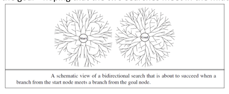
Bidirectional Search

Run two simultaneous searches, one forward from the initial states and the other backward from the goal, hoping the two searches meet in the middle

Implemented by replacing the goal test with a check to see whether the frontiers of the 2 searches intersect, if they do a solution has been found

Weakness is the space requirement

Uninformed Search Methods

Have access only to the problem definition

BFS: Expands the shallowest nodes first; complete, optimal for unit sep costs, exponential space complexity

Dijkstra: Uniform cost search expands the node with lowest path cost, g(n), and is optimal for general step cost

DFS: Expands the deepest unexpanded node first, incomplete, not optimal, has linear space complexity

Informed Search Methods

May have access to a heuristic function h(n), estimates the cost of a solution from n

Greedy best first search: Expands nodes with minimal h(n), not optimal but most efficient, f(n) = h(n)

A\* search: Expands nodes with minimal f(n) = g(n) + h(N), complete and optimal, space complexity is prohibitive

Adversarial Games

Competitive environments, in which the agents' goals are in conflict
Deterministic, fully oberservable environments where 2 agent act alternately and in which the utility value at the end of the game are always equal and opposite

Cooperative Game

Players should adopt a certain strategy through negotiations and agreements between players

Non-cooperative game

Game where players cannot form alliances or if all agreements need to be self-enforcing

Symmetric Game

Game where the payoffs for playing a particular strategy depend only on the other strategies employed, not on who is playing them

Asymmetric Game

Game where each player begins the game differently than everyone else
While the winning conditions are the same for everyone, each player will be pursuing very different paths to achieve that goal

Zero sum game

Game where choices by players can neither increase nor decrease the available resources
Total benefit goes to all players in a game, for every combination of strategies, always adds to zero (more informally, a player benefits only at the equal expense of others)

Simultaneous game

Games where both players move simultaneously, or instead the later players are unaware of the earlier players' actions

Sequential Games

Also known as dynamic games
Games where later players have some knowledge about earlier actions. This need be perfect information about every action of earlier players; might be very little knowledge
A player may know that an earlier player did not perform one particular actions, while they do not know which of the other available actions the first player performed

Perfect Information

A game where all players, at every move in the game, know the moves previously made by all other players
Example: Firms and consumers having information about the price and quality of all the available goods in a market, Tic Tac Te, checkers, chess

Imperfect Information

A game where the players do not know all moves already made by the opponent such as a simultaneous move game
Example: Many card games

Game Definition

Games with 2 players (MAX and MIN)
MAX moves first and then they take turns moving until the game is over. At the end of the game, points are awarded to the winning player and penalties to the loser
Game has s_0, Player(s), Action(s), Result(s, a), Terminal-Test(s), and Utility(s, p)

s_0

The initial state of a game
Specifies how the game is set up to start

Player(s)

Defines which player has the move in a state of a game

Actions(s)

Returns the set of legal moves in a state of a game

Terminal-Test(s)

A terminal test, which is true when the game is over and false otherwise
States where the game has ended

Utility(s, p)

A utility function (also called objective function or payoff function) defines the final numeric value for a game that ends in terminal state s for a player p

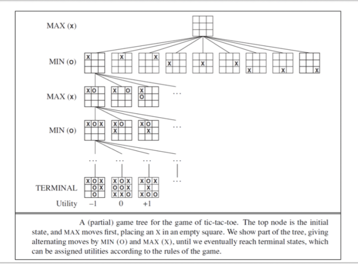
Game Tree

ACTIONS function and RESULT function define this of a game
A tree where the nodes are game states, and the edges are moves

Tic Tac Toe

From the initial state, MAX has 9 possible moves
Game tree is relatively small - fewer that 9! \= 262, 880 terminal nodes

Optimal Decision

In adversarial search, MIN has something to say about finding the sequence of actions leading to a goal state
MAX must find a contingent strategy that specifies MAX's moves in the initial state, then MAX's moves in the states resulting from every possible response by MIN, then MAX's moves in the states resulting from every possible response by MIN to those moves
Leads to outcome at least as good as any other strategy when one is playing an infallible opponent

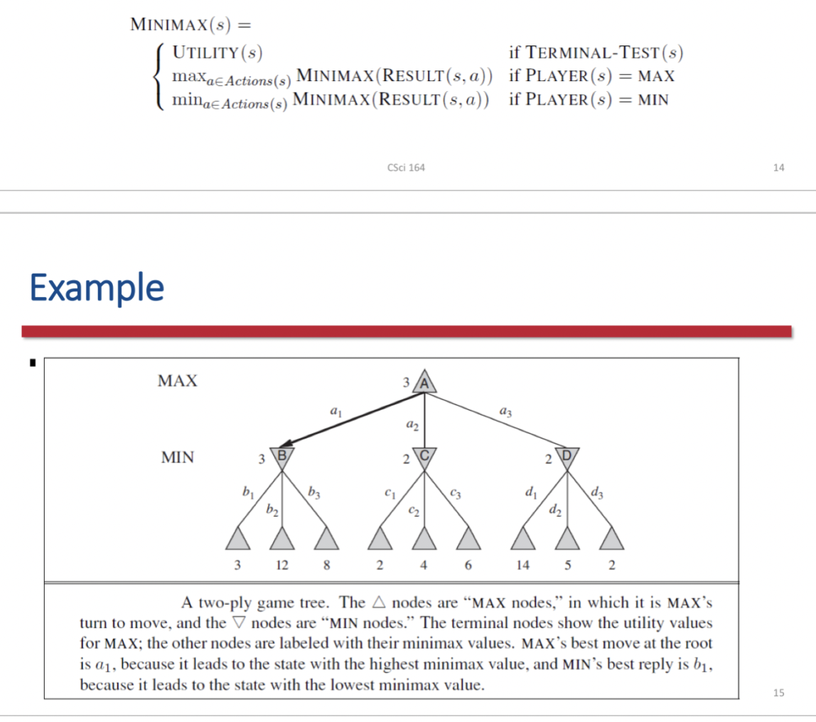
Minimax

Given a game tree, the optimal strategy can be determined from the minimax value of each node, which we write as MINIMAX(n)
The minimax value of a node is the utility (for MAX) of being in the corresponding state, assuming that both players play optimally from there to the end of the game
Minimax value of a terminal state is just it's utility
Given a choice, MAX prefers to move to a state of maximum value, whereas MIN prefers a state of minimum value

Minimax Algorithm

Computers the minimax decision from the current state
Recursion proceeds all the way down to the leaves of the tree, and then the minimax values are backed up through the tree as the recursion unwinds
Performs a complete depth-first exploration of the game tree

O(b^m)

The maximum depth of the game tree is m and there are b legal moves
Time complexity of the minimax algorithm

O(bm)

The maximum depth of the game tree is m and there are b legal moves
Space complexity for a minimax algorithm that generates all actions at once

O(m)

The maximum depth of the game tree is m and there are b legal moves
Space complexity for a minimax algorithm that generates actions one at a time

Minimax Search

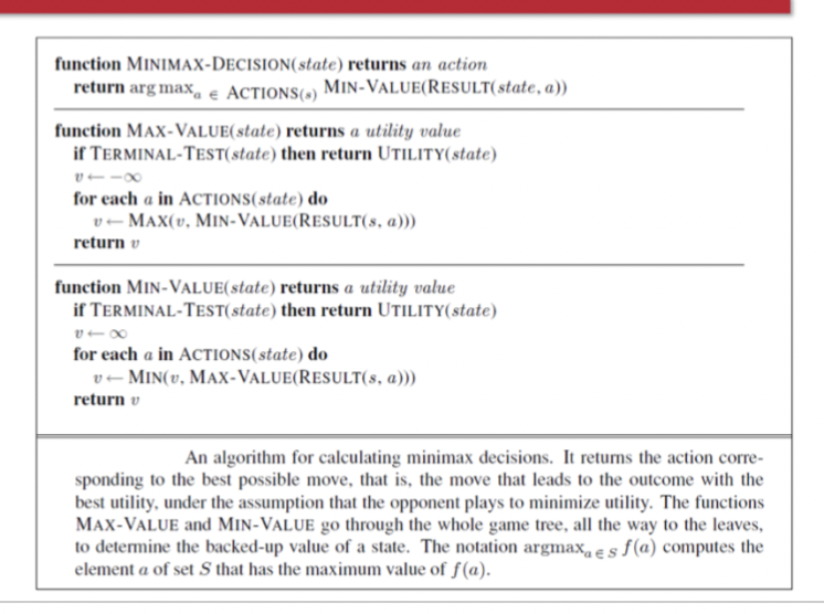
Algorithm for calculating the optimal move using minimax
The move that leads to a terminal state with maximum utility, under the assumption that the opponent plays to minimize utility
The functions MAX-VALUE and MIN-VALUE go through the whole game tree, all the way to the leaves, to determine the backed-up value of a state and the move to get there
Problem: Number of game states it has to examine is exponential in the depth of the tree

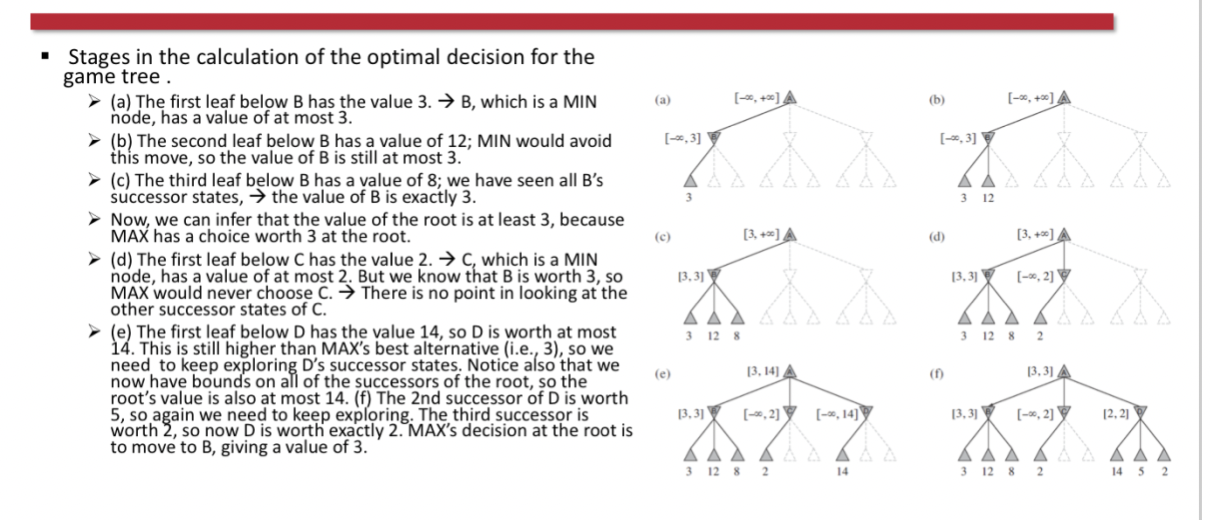
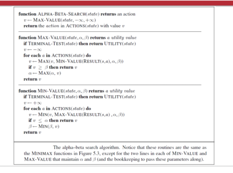
Alpha-beta Pruning

Rationale: Minimax Search has to examine an exponential number of game states, thus want to prune to eliminate large parts of the tree from consideration
Returns the same move as minimax would but prunes away branches that cannot possibly influence the final decision
Can be applied to trees of any depth, often possible to prune entire subtrees rather than just leaves
Effectiveness is highly dependent on the order in which the states are examined

Alpha-beta Search

Same as MINIMAX SEARCH functions, expect that we maintain bounds in the variables 𝛼 and 𝛽, and we use them to cut off search when a value is outside the bounds
General principle:
- Consider a node n somewhere in the tree such that Player has a choice of moving to that node
- If player has a better choice m either at the parent node of n or at any choice point further up, then n will never be reached in actual play
- Once we have found out enough about n (by examining some of its descendants) to reach this conclusion we can prune it
Updates the values of 𝛼 and 𝛽 as it goes along and prunes the remaining branches at a node (i.e. terminates the recursive call) as soon as the value of the current node is known to be worse that the current 𝛼 or 𝛽 value for MAX or MIN, respectively

alpha

In alpha-beta search it is the value of the best (i.e highest value) choice we have found so far at any choice point along the path for MAX

beta

In alpha-beta search it is the value of the best (lowest-value) choice we have found so far at any choice point along the path for MIN

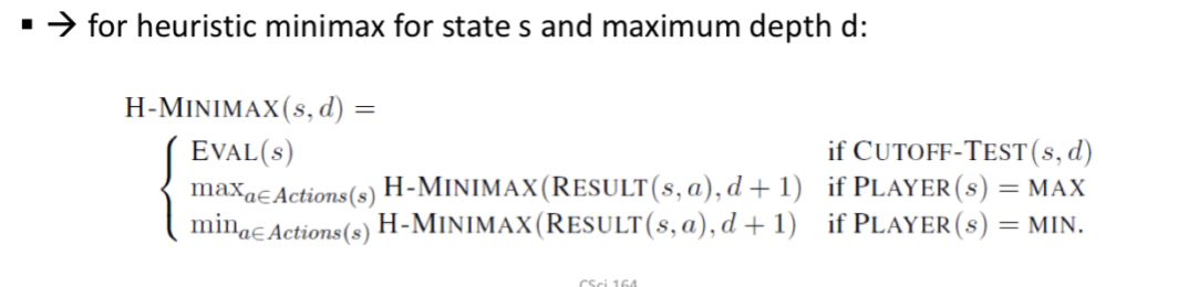
Imperfect Real Time Decision

Programs should cut off the search earlier and apply a heuristic evaluation function into states in the search, effectively turning nonterminal nodes into terminal leaves
Suggestion is to alter minimax or alpha-beta pruning in 2 ways:
1) Replace the utility function by a heuristic evaluation function EVAL, which estimates the position's utility
2) Replace the terminal test by a cutoff test that decides when to apply EVAL
Psedocode:
If the search must be cut off at nonterminal states then the algorithm will necessarily be uncertain about the final outcomes of those states
- This type of uncertainty is induced by computation, rather than information, limitations
Determine the value of the current state of the game

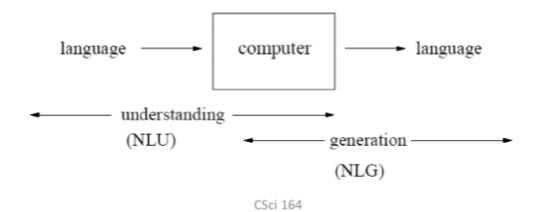
Natural Language Processing (NLP)

Field in AI for creating computers that use natural language as input and/or output
Kind of translator between humans and machines
To interact with computing devices using human (natural language)
To access (large amount of) information and knowledge stored in the form of human languages quickly
Ex: Enables auto suggestion, chatbots

Text Analytics

Involves the extraction of limited kinds of semantic and pragmatic information from texts

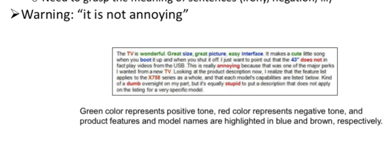
Sentiment Analysis

Deals with categorization (or classification) of opinions expressed in textual documents

NLP Tasks

NLP applications require several NLP analyses
- Work tokenization
- Sentence boundary detection
- Part-of-speech (POS) tagging
- Named Entity (NE) recognition
- Parsing
- Semantic Analysis

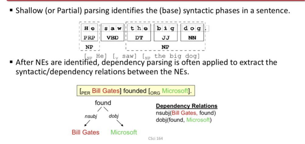
Shallow Parsing

Identifies the (base) syntactic phrases in a sentence
After NEs identified, dependency parsing is often applied to extract the syntactic/dependency relations between the NEs