CFA Level 1 (Formulas/Main Concepts)

Future Value (FV) of a Single Cash Flow

FV = PV x (1+r)^n

where PV is the present value, r is the interest rate, and n is the number of periods.

Present Value (PV) of a Single Cash Flow

PV = FV / (1+r)^n

where FV is the future value, r is the interest rate, and n is the number of periods.

Present Value (PV) of Perpetuity

PV (perpetuity) = A / r

A= payment amount

Effective Annual Rate (EAR)

EAR = (1 + Periodic Rate)^m - 1

Periodic Rate = State Annual Rate / Number of Compounding Periods One Year

m = Number of Compounding Periods One Year

Arithmetic Mean

Sum of all observation values in sample/population, divided by # of observations

Geometric Mean

G_r = [(1+R₁) x … x (1+R_n)^(1/n) - 1

Harmonic Mean

Harmonic Mean = N / Σ(1/x_i)

ex. N/(1/x₁)x(1/x₂)

Largest to Smallest of Quant Means

Arithmetic > Geometric > Harmonic

Skew and Mean/Median/Mode Relationship

Negative Skew: Mean < Median < Mode

Positive Skew: Mean > Median > Mode

In a negatively skewed distribution, the mean is less than the median, which is less than the mode, whereas in a positively skewed distribution, the mean is greater than the median, which is greater than the mode.

Weighted Average Mean

X_w = ∑ W_i x X_i

Mean Absolute Deviation

MAD = ∑ | X_i - X̄| / n

Percentile

Percentile = Ly = (n + 1) x (y/100)

Quartile = Distribution / 4

Quintile = Distribution / 5

Decile = Distribution / 10

Trimmed Mean

A trimmed mean is a statistical measure that adjusts the mean by removing a specified percentage of the lowest and highest values from a dataset, providing a more robust estimate of central tendency. This helps mitigate the influence of outliers.

Winsorized Mean

A Winsorized mean is a statistical measure that limits extreme values in the dataset to reduce the impact of outliers, typically by replacing the smallest and largest values with the nearest remaining values.

Population Variance

σ² = ∑ (x_i - μ)² / N

Sample Variance

S² = ∑ (x_i - X̄ )² / (n - 1)

Target Downside Deviation (Semi - Deviation)

S_Target = √(∑ ( X_i - target)² / n-1)

The sum of the numerator and denominator together is used to calculate the average of squared deviations from the specified target, providing a measure of downside risk.

Coefficient of Variation

CV = Standard Deviation of x / Average Value of x

CV = S_x / X̄

Coefficient of Variation: expresses how much dispersion exists relative to mean of a distribution; allows for direct comparison of dispersion across different data sets. CV is calculated by dividing standard deviation of a distribution by the mean or expected value of the distribution

Probability of A or B

P (A or B) = P(A) + P(B) - P(AB)

Joint Probability of Two Events

P(AB) = P(A|B) x P(B)

Conditional Probability of A given B

P(A|B) = P(AB) / P(B)

Expected Return (expected value of a random variable)

E(X) = ∑ P(X₁)X₁

_{E(X) =} P(X₁)X₁ + P(X₂)X₂ +…+ P(X_n)X_n

Expected Variance (square root for std.dev.) / Probabilistic Variance

σ²(X) = ∑ P(X_i) [X_i - E(X)]²

σ²(X) = P(X₁) [X₁ - E(X)]² + P(X₂) [X₂ - E(X)]² …

Portfolio Expected Return

E(R_p) = w_AE(R_A) + w_BE(R_B)

Just R instead of E(R) if its actual returns

Portfolio Variance

Var(R_P) = (w_A² x σ²(R_A)) + (w_B² x σ²(R_B)) + 2w_Aw_Bσ(R_A)σ(R_B)ρ(R_A,R_B)

Correlation

corr(R_i,Rj) = Cov(Ri,Rj) / (σ(Ri)σ(Rj))

Covariance

cov(X_i,Y_j) = E[X_i - E(X_i) (Y_j - E(Y_j)]

Roy’s Safety - First Ratio

= r̄_p - r_target / σ_p

Portfolio with the highest ratio is preferred

Log Lin Model

ln(y_i) = b₀ + b₁(x_i) + ε (error term)

Relevant change in the dependent variable and an absolute change in the independent variable

Lin Log Model

y_i = b₀ + b₁(ln(x_i)) + ε (error term)

Absolute change in the dependent variable and a relative change in the independent variable

Log Log Model

ln(y_i) = b₀ + b₁(ln(x_i)) + ε (error term)

Relative change in boththe dependent and independent variables.

Beta

Beta_i = cov_i,mkt / var_mkt

Joint Probability of any number of independent events

P(ABCDE) = P(A) x P(B) x P(C) x P(D) x P(E)

Bayes Formula

P(Event | Information) = [ P(Information | Event) / P(Information) ] x P(Event)

Normal Distributions

Normal Distribution is completely described by its mean and Variance

68% of observations fall with ± 1σ

90% of observations fall with ± 1.65σ

95% of observations fall with ± 1.96σ

99% of observations fall with ± 2.58σ

Computing Z - Scores

x - μ / σ

Degrees of Freedom of a Students’ T-distribution

df = number of sample observations -1 = n-1

Central Limit Theorem

When selecting simple random samples of size n from population with mean µ and finite variance σ2 , the sampling distribution of sample mean approaches normal probability distribution with mean µ and variance equal to σ2 /n as the sample size becomes large.

Standard Error the Sample Mean

Standard error of the sample mean is the standard deviation of distribution of the sample means.

known population variance: σ_x = σ / √n

unknown population variance: S_x = S / √n

Resampling Techniques (Jackknife and bootstrap)

Jackknife: Calculate multiple sample means, each with one observation removed, the calculate standard deviation of the sample means

Bootstrap: Draw repeated samples of size n from the full dataset, replacing the sampled observations each time, then calculate the standard deviation of the sample means

Null and Alternative Hypothesis

Null Hypothesis (H_o) : hypothesis that contains the equal sign (=, <=, >=)

Alternative Hypothesis (H_A) : concluded if there is sufficient evidence to reject the null hypotheses

Type I and Type II Errors

Type I Error = rejecting the null hypothesis when it is true

Type II Error = failing to reject the null hypothesis when it is false.

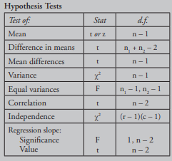
Hypothesis Tests

Power of a Test

1 - P(Type II Error)

Significance Level

Given a significance level of 5% (Confidence interval 95%), a test will reject a true null hypothesis 5% of the time

Regression Coefficient

Y = b₀ +b₁X₁ + ε_i

Where:

Y= Dependent Variable

X= Independent Variable

b₀ = Intercept Term

b₁ = Slope Term

ε = Error Term (Residual)

Estimated Intercept and Slope Terms

b₀ = ȳ - b_ix̄

b₁ = COV_XY / σ²_X

Analysis of Variance (ANOVA)

Total sum of squares (SST) = sum of squared differences between actual Y-values and the mean of Y

Sum of squares regression (SSR) = sum of squared distances between predicted Y-values and the mean of Y

Sum of squared errors (SSE) = sum of squared distances between actual and predicted Y-values

Coefficient of Determination

Coefficient of Determination R₂ = SSR/SST = percentage of variation in the dependent variable explained by variation in the independent variable

Explained Variance / Total Variance

Assumptions of Simple Linear Regression (Linearity, Homoscedasticity, Independence, Normality)

Linearity: A linear relation exists between the dependent variable and the independent variable

Homoscedasticity: Variance of the error term is the same for all observations

Independence: The error term is uncorrelated across observations

Normality: the error term is normally distributed

TSS (total sum of squares)

TSS = SSE + RSS

SSE: sum of the squared errors (unexplained variance)

RSS: regression sum of squares (explained variance)

Breakeven and Shutdown Points

Breakeven Point: Total Revenue = Total Cost

Shutdown Point (short run): Total Revenue < Total Variable Cost

Shutdown Point (long run): Total Revenue < Total Cost

Market/Firm Structures

Perfect competition: Many firms with no pricing power; very low or no barriers to entry; homogeneous product.

Monopolistic competition: Many firms; some pricing power; low barriers to entry; differentiated products; large advertising expense.

Oligopoly: Few firms that may have significant pricing power; high barriers to entry; products may be homogeneous or differentiated.

Monopoly: Single firm with significant pricing power; high barriers to entry; advertising used to compete with substitute products. In all market structures, profit is maximized at the output quantity for which marginal revenue = marginal cost

Profit Maximization Point (All Firms)

Marginal Revenue = Marginal Cost

Gross Domestic Product (GDP)

GDP Expenditure Approach) = Consumption + Investments + Government Spending + New Exports

GDP (Income Approach) = Household Income + Business Income + Government Income

GDP ( Value-Added Approach): Sum incremental value-added at each stage of production

Nominal and Real GDP

Nominal GDP = (Deflator x Real GDP) / 100

Real GDP = Nominal / Deflator

GDP Deflator = (Value of current year output at current prices / Value of current year output at base year prices) x 100

Savings, Investments, Fiscal Balance, and Trade Balance

Fiscal budget deficit (G - T) = excess of saving over domestic investments (S - I) - trade balance (X - M)

S= Private Savings

I= Gross private domestic investment. It consists of business investments in capital goods as well as inventory changes.

G= Government expenditure on finished goods and services

X= Export

M= Imports

Aggregate Demand and Supply

AD: shifts due to changes in household wealth, consumer and business expectations, capacity utilization, monetary policy, fiscal policy, exchange rates and foreign GDP

AS:

Short-Run Shifts: changes in changes in potential GDP, nominal wages, input prices, future price expectations, business taxes and subsidies and exchange rate

Long-Run Shifts: changes in labor supply, supply of physical and human capital and productivity and technology

Growth Accounting Equation

Growth in Potential GDP = growth in technology + growth in labor + growth in capital

Business Cycles

Trough (lowest point); expansion; peak (highest point); contraction

Expansion: Rising GDP, decreasing unemployment,

Credit Cycles

Tend to amplify business cycles, and do not coincide (tend to last longer)

Characteristics of the 4 Stages of the Business Cycle

• Trough:

  • The GDP growth rate changes from negative to positive.

  • There is a high unemployment rate, and an increasing use of overtime and temporary workers.

  • Spending on consumer durable goods and housing may increase.

  • There is a moderate or decreasing inflation rate.

• Expansion:

  • The GDP growth rate increases.

  • The unemployment rate decreases as hiring accelerates.

  • There are investment increases in producers' equipment and home construction.

  • The inflation rate may increase.

  • Imports increase as domestic income growth accelerates.

• Peak:

  • The GDP growth rate decreases.

  • The unemployment rate decreases, but hiring slows.

  • Consumer spending and business investments grow at slower rates.

  • The inflation rate increases.

• Contraction/recession:

  • The GDP growth rate is negative.

  • Hours worked decrease; unemployment rate increases.

  • Consumer spending, home construction, and business investments decrease.

  • The inflation rate decreases with a lag.

  • Imports decrease as domestic income growth slows.

Economic Indicators

Leading: Turning points occur ahead of peaks and troughs (S&P 500, manufacturing new orders, building permits)

Coincident: Turns coincide with peaks and troughs (employee payrolls, manufacturing sales, personal income)

Lagging: Turns after peaks and troughs (average prime rate, inventory-sales ratio, duration of unemployment)

Types of Unemployment

Frictional: Unemployment from time lag to find new job

Cyclical: Unemployment due to business cycle fluctuations

Structural: Unemployment due to lack of skills for job openings or distance factors

Consumer Price Index (CPI)

CPI =( Cost of basket at current prices / cost of basket at base period prices) x 100

Monetary Policy (expansion vs contraction)

Central bank activities that influence the supply of money and credit;

expansionary when policy rate < neutral interest rate

contractionary when policy rate > neutral interest rate

Central Bank Objectives

Full employment and Price Stability

Money Multiplier

= 1 / reserve requirement

Fiscal Policy

Fiscal Policy: government decisions about taxation and spending

expansionary when a budget deficit is increasing or surplus is decreasing

contractionary when a budget deficit is decreasing or a surplus is increasing

Fiscal Multiplier

= 1/ 1 - MPC(1-t)

Balance of Payments

Current account: measures flow of goods and services (merchandise and services; income receipts; unilateral transfers)

Capital account: measures transfers of capital (capital transfers; sales/purchases of nonfinancial assets)

Financial account: records investment flows (government-owned assets abroad; foreign-owned assets in the country)

Regional Trade Agreements

Free trade area: Removes barriers to goods and services trade among members.

Customs union: Members also adopt common trade policies with non-members.

Common market: Members also remove barriers to labor and capital movements among members.

Economic union: Members also establish common institutions and economic policy.

Monetary union: Members also adopt a common currency

Exchange Rate

Price Currency / Base Currency

(base is 1)

Real Exchange Rate

Nominal FX rate x [(base currency CPI) / (price currency CPI)]

No-Arbitrage Forward Exchange Rate

= Spot Rate x [(1 + price currency interest rate) / (1 + base currency interest rate)]

Exchange Rate Regimes

Formal dollarization: country adopts foreign currency.

Monetary union: members adopt common currency.

Fixed peg: ±1% margin versus foreign currency or basket of currencies.

Target zone: Wider margin than fixed peg.

Crawling peg: Pegged exchange rate adjusted periodically.

Crawling bands: Width of margin increases over time.

Managed floating: Monetary authority acts to influence exchange rate but does not set a target.

Independently floating: Exchange rate is market determined

Financial Statement Analysis Framework

1. State the objective and context

2. Gather data

3. Process the data

4. Analyze and interpret the data

5. Report conclusions or recommendations

6. Update the analysis

Auditors Opinion

Unqualified (unmodified, clean): Reasonable assurance that financial statements are free from material omissions and errors.

Qualified: Exceptions to accounting principles.

Adverse: Statements are not presented fairly or do not conform with accounting standards.

Disclaimer of opinion: Auditor is unable to express an opinion.

Revenue Recognition Principles

Requirements: 1) risk and reward of ownership is transferred, 2) collectability is probable

Five-step revenue recognition model:

1. Identify contracts

2. Identify performance obligations

3. Determine transaction price

4. Allocate price to obligations

5. Recognize when (as) obligations are satisfied

Expense Recognition Principles (matching)

Matching Principle: Match expenses with the revenues they help generate

Basic Earnings Per Share (EPS)

Basic EPS = (net income - preferred Dividends) / Weighted average # of common shares outstanding

Diluted EPS

Diluted EPS = (adj. income avail. for common shares) / ( wtd. avg. common shares plus potential common shares outstanding)

Diluted EPS = [(net income - pfd div) + convertible preferred dividends − (convertible debt interest) x (1-t)] / ([wtd. avg shares)+ shares from conversion of conv. pfd. share) + (shares from conversion conv debt) + (shares issuable from stock options)]

Marketable Security Classifications

Held-for-trading: fair value on balance sheet; dividends, interest, realized and unrealized G/L recognized on income statement.

Available-for-sale: fair value on balance sheet; dividends, interest, realized G/L recognized on income statement; unrealized G/L is other comprehensive income.

Held-to-maturity: amortized cost on balance sheet; interest, realized G/L recognized on income statement.

Comprehensive Income

= Net Income + Other Comprehensive Income

IFRS vs U.S. GAAP

IFRS

Interest Received: Operating or Investing

Interest Paid: Operating or Financing

Dividends Received: Operating or Investing

Dividends Paid: Operating or Financing

U.S. GAAP

Interest Received: Operating

Interest Paid: Operating

Dividends Received: Operating

Dividends Paid: Financing

Cash Flows from Operations (CFO)

Direct method: start with cash collections (cash equivalent of sales); cash inputs (cash equivalent of cost of goods sold); cash operating expenses; cash interest expense; cash taxes.

Indirect method: start with net income, subtracting back gains and adding back losses resulting from financing or investment cash flows, adding back all noncash charges, and adding and subtracting asset and liability accounts that result from operations

Increase in a Current Asset: -

Decrease in a Current Asset +

Increase in a Current Liability: -

Decrease in a Current Liability: +

Free Cash Flow (FCF)

Free Cash Flow (FCF) measures cash available for discretionary purposes and is equal to operating cash flow less net capital expenditures

Free Cash Flow to the Firm (FCFF)

FCFF = NI + NCC + Int(1 - tax rate) - FCInv - WCInv

FCFF = CFO + Int(1 - Tax rate) - FCInv

NCC = Net Noncash Charges

FCInv = Fixed Capital Investments

WCInv = Working Capital Investments

Free Cash Flow to Equity (FCFE)

FCFE = CFO - FCInv + Net Borrowing

FCFE = NI + NCC - CapEx - ∆Working Captital + Net Borrowing

NCC = Net Noncash Charges

FCInv = Fixed Capital Investments

Common-Size Financial Statement Analysis (Balance Sheet, Income Statement, Cash Flow Statement)

Common size balance sheet expresses all balance sheet accounts as a percentage of total assets

Common size income statement expresses all income statement items as a percentage of sales

Common size Cash Flow Statement expresses each line item as a percentage of net revenue

Horizontal common-size financial statements analysis expresses each line item relative to its value in a common base period

Liquidity Ratios: Current Ratio, Quick Ratio, Cash Ratio

Current Ratio = current assets / current liabilities

Quick ratio = cash + marketable securities + receivables / current liabilities

Cash Ratio = Cash + marketable securities / current liabilities

Defense Interval

Defense Interval = cash + mkt. sec. + receivables / daily cash expenditures

Cash Conversion Cycle

CCC = DOH + DSO - DPO

where DOH is Days of Inventory Held, DSO is Days Sales Outstanding, and DPO is Days Payable Outstanding.

Receivables Turnover

Days Sales Outstanding (DSO)

Receivables Turnover = Annual sales / average receivables

DSO = 365 / Receivables turnover

Inventory Turnover

Days Inventory on Hand

Inventory Turnover = COGS / average inventory
Days Inventory on Hand = 365 / Inventory Turnover

Payables Turnover Ratio

Number of Days Payables

Payables Turnover Ratio = Cogs / Average Payables

DPO = 365 / Payables turnover ratio

Total Asset Turnover

Fixed Asset Turnover

Working Capital Turnover

Total asset turnover = Revenue / average total assets

Fixed asset turnover = Revenue / average fixed assets

Working capital turnover = Revenue / average working capital

Gross Profit Margin

Operating Profit Margin

Net Profit Margin

ROA

ROE

Gross profit margin = gross profit / revenue

operating profit margin = operating profit / revenue = EBIT / net sales

net profit margin = net income / revenue

ROA = net income / average total assets
ROE = net income / average total equity

Return on Total Capital (ROTC)

return on assets (total capital) = EBIT / average total capital

Debt to assets (total debt) ratio

Debt to equity ratio

Financial leverage

Debt - Assets = Total Debt / Total Assets

Debt - Equity = Total Debt / Total Equity

Financial Leverage = Total Assets / Total Debt