Graph Algorithms

Explain the basic graph concepts: path, cycle, cyclic/acyclic graph

Path

A path from v1 to vn is a sequence
v1 v2 ... vn
such that every next vertex is reachable by an edge.

Example:
Edges: a -> b, b -> c
Path: a b c

A simple path means no vertex repeats.

---

Cycle
A cycle is a simple path that comes back to the start.

Example:
a -> b -> c -> a

---

Cyclic / Acyclic graph

• Cyclic: has at least one cycle

• Acyclic: no cycles

What is strongly connected graph, strongly connected component (SCC),

For every pair u , v, there is:

• a path from u to v

• and a path from v to u

Example:
a -> b -> c -> a
All nodes reach each other → strongly connected

---

Connected (directed)
Ignore direction by adding reversed edges.
If the result is strongly connected → graph is connected.

Reversed edges set:
ET = {(v, u) | (u, v) in E}

---

Strongly Connected Component (SCC)
A maximal set of vertices where:

• every vertex reaches every other

Think: “islands” of strong connectivity.

What are the basic operations a graph data structure should support?

successor = neighbour

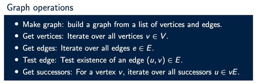
If v = a (Vertex is a) and edges are a -> b, a -> c
Then aE = {b, c}

So aE contains only vertices you can reach in ONE edge from a.

What are adjacency lists and adjacency matrices, and when should each be used?

Adjacency list
For each vertex v, store a list of successors vE.

Example:

0: [1, 3]
1: [2]
2: []
3: [2]

---

Adjacency matrix
A 2D table where entry (u, v) is:

• true if edge exists

• false otherwise

Example:

    0 1 2
0 [ 0 1 0 ]
1 [ 0 0 1 ]
2 [ 0 0 0 ]

Adjacency list (usually better)

• Memory efficient

• Fast iteration over neighbors

• Best for sparse graphs

---

Adjacency matrix preferred if

• Graph is dense
  (|E| close to |V|^2)

• Edge existence tests are very frequent

• Performance difference doesn’t matter

How does edge testing and edge iteration work using an adjacency matrix?

Data Structure:

The graph stores:

• number of vertices n

• matrix adj_matrix[u][v]

---

Edge test

Check directly: adj_matrix[u][v] = true
means edge (u, v) exists

Time: O(1)

---

Iterate over all edges: List all edges (u, v) that actually exist in the graph.

Because every edge is stored as one cell in the matrix, we must:

1. Look at every row u

2. Look at every column v

3. Check whether adj[u][v] is true

4. If yes → (u, v) is an edge

How does edge testing and edge iteration work using an adjacency list?

For each vertex u:

• store a list adj_list[u] of neighbors.

• with its size

Example:

0: [1, 3]
1: [2]
2: []
3: []

Edge test

Check if v is inside adj_list[u]:

adj_list[u].contains(v)

Time:

• worst case: O(deg(u))

• can be improved with binary search or hash table

---

Iterate over all edges

Steps:

1. For each u

2. For each v in adj_list[u]

3. Output (u, v)

Total time:
O(|V| + |E|) -> is faster

What is graph traversal, and what is it used for?

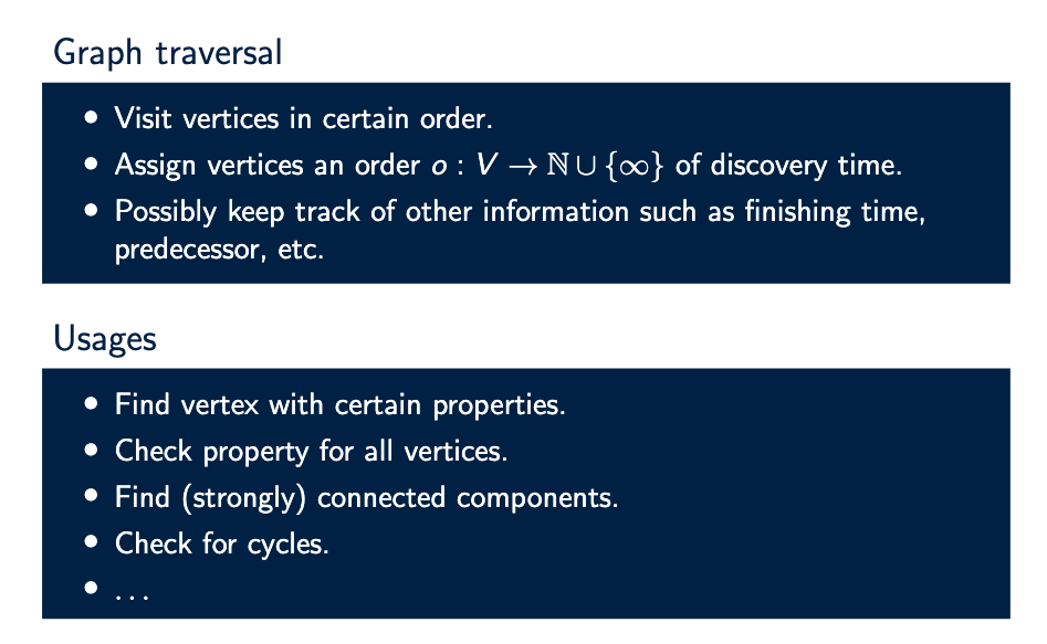
What is the basic idea of Depth First Search (DFS)?

Depth First Search (DFS) explores the graph:

as deep as possible before backtracking

Key idea:

• use a stack to store vertices that still need exploration

Steps (high level):

1. Start from a vertex

2. Go to one of its successors

3. Keep going deeper

4. If no unvisited successor exists → go back

This is why it’s called depth-first.

DFS algorithm steps

We explain DFS using:

• a stack S

• a discovery order o(v)

Initially:

for all v:
  o(v) = ∞

---

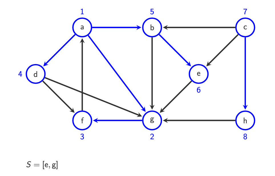
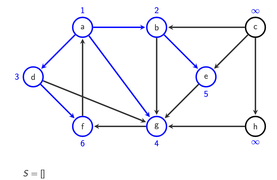
Step 1 — Start

• Choose a start vertex (e.g. a)

• Push it onto the stack

S = [a]

---

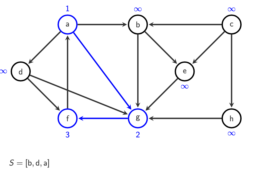
Step 2 — Pop & discover

• Pop top of stack

• If not visited (o(v) = ∞), assign next number

Example:

o(a) = 1

---

Step 3 — Push successors

• Push all successors of a onto the stack

Example:

a -> b, d, g
S = [b, d, g]

(Exact order depends on implementation)

---

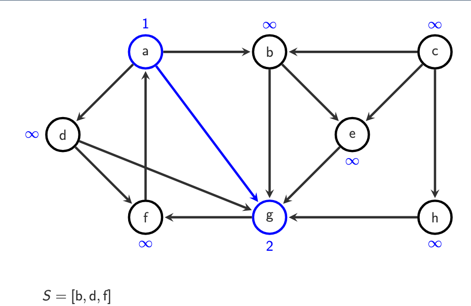
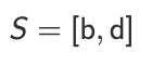
Step 4 — Repeat

Repeat while stack is not empty:

1. Pop a vertex v

2. If o(v) = ∞, assign next number &

   1. Push all successors of v

---

Key observation (VERY IMPORTANT)

• A vertex can be pushed multiple times

• It is only processed once

• The check o(v) = ∞ prevents revisiting

---

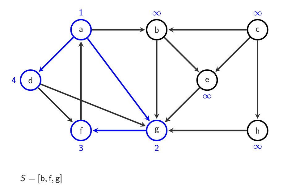
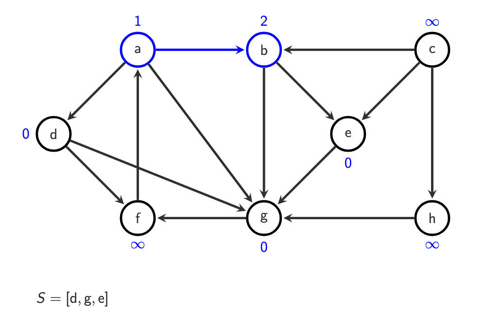
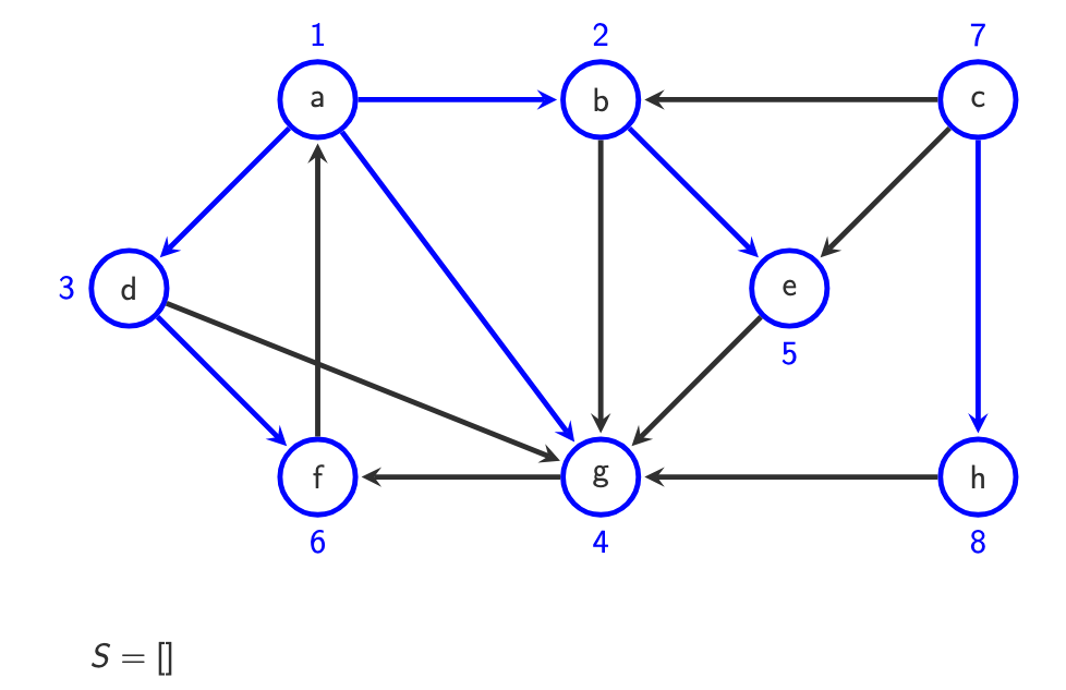
When DFS ends

DFS finishes when

S = []

& only after we tried every vertex in V and its oo(v) ≠ ∞

DFS procedure

Main loop

For each vertex v:

• if o(v) = ∞, start DFS from v

---

DFSExplore procedure

push v onto S
while S not empty:
  v = pop S
  if o(v) = ∞:
    o(v) = i
    i = i + 1
    for each u in vE:
      push u onto S

---

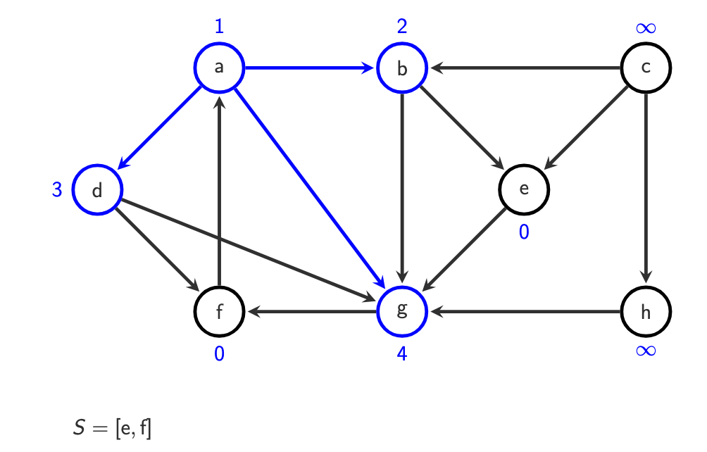
Running time

Each vertex and edge is processed at most once:

O(|V| + |E|)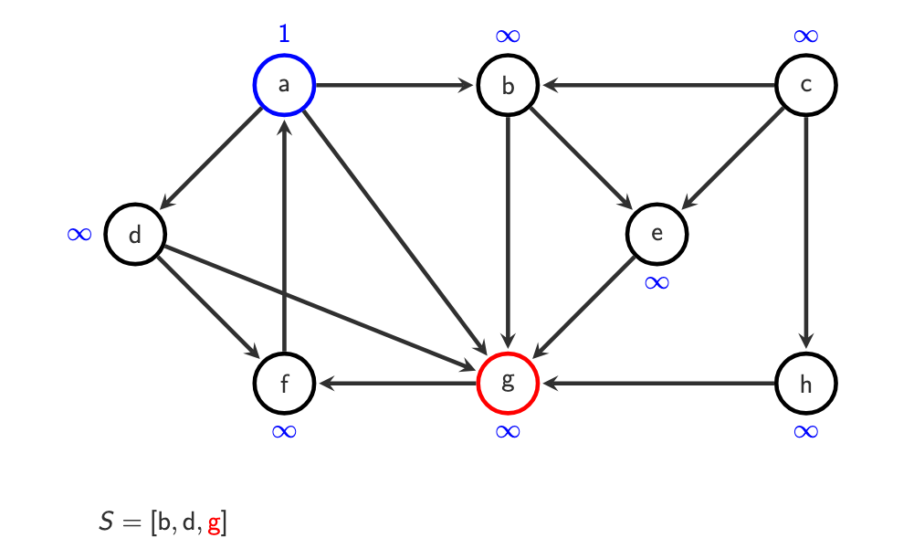

…

S= [] finished and all vertices visited.

How can DFS be used to detect cycles?

DFS detects cycles by looking for back edges.
A back edge is an edge to a vertex that is already on the current DFS path. (in the stack, waiting)
If such an edge exists, the graph contains a cycle.
In undirected graphs, the edge to the predecessor is ignored.

What is the basic idea of Breadt First Search (BFS)?

Breadth First Search (BFS) explores the graph:

level by level, starting from a source vertex.

Key difference to DFS:

• DFS → stack → goes deep

• BFS → queue → stays shallow first

So BFS visits:

• all vertices at distance 1

• then distance 2

• then distance 3

• etc.

Start from vertex a.

Step 1 — start

S = [a]
o(a) = 1

Step 2 — visit neighbors of a

From a, we discover:

b, d, g

They are:

• marked as discovered

• put into the queue

S = [b, d, g]
 

Step 3 — process queue in order

Important:

• they are all distance 1 from a

Now BFS continues:

• dequeue b

• enqueue undiscovered neighbors of b

Then:

• dequeue d

• then g

• then their neighbors

So the queue ensures:

vertices discovered earlier are processed first

This guarantees level-by-level traversal.

When a vertex u is discovered:

o(u) = 0

This marks it as:

• discovered

• but not fully processed yet

BFS procedure

Main procedure

for each v:
  o(v) = ∞

S = empty queue
i = 1

for each v:
  if o(v) = ∞:
    BFSExplore(v)

---

BFSExplore procedure

enqueue v into S

while S not empty:
  v = dequeue S
  o(v) = i
  i = i + 1

  for each u in vE:
    if o(u) = ∞:
      o(u) = 0
      enqueue u into S

---

Running time

Each vertex and edge is handled a constant number of times:

O(|V| + |E|)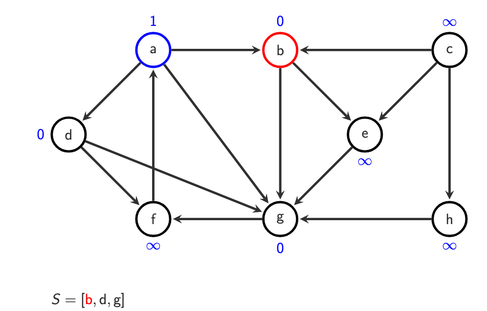

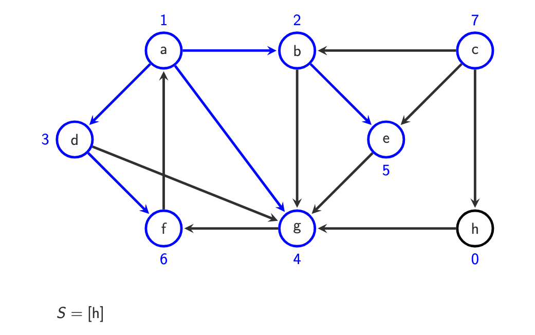
g is visited, because it’s 0 we do with g afterwards:

do with c afterwards, it has infinity. Its neighbour is h, we put it in.

Why is BFS suitable for finding shortest paths in unweighted graphs? BFS limitiation

Key observation:

The queue in BFS is automatically ordered by distance from the source.

Because:

• vertices at distance k are discovered before

• vertices at distance k+1

reconstruct shortest paths by storing predecessors

BFS works for:

• unweighted graphs

• or graphs where all edges have equal weight

For weighted graphs with non-negative weights:

• BFS generalizes to Dijkstra’s algorithm

• which uses a priority queue instead of a FIFO queue

What is a topological order, and when does it exist?

A topological order is an assignment of numbers to vertices:

o : V -> N

such that for every directed edge: (u, v) in E

we have:

o(u) < o(v)

Meaning:

• u must come before v in the order

A topological order exists if and only if the graph is a DAG (directed acyclic Graph)

Important notes

• A topological order is not unique

• Multiple valid orders may exist

What are typical applications of topological sorting?

Topological sorting is used when there are dependencies.

Typical examples:

• task scheduling

• instruction ordering

• resolving dependencies (e.g. build systems)

• Detecting cycles.

• Find shortest paths from a source in some weighted DAG in linear time.

Explain the idea of topological sort using predecessor counts.

For every vertex v, compute:

pre(v) = number of incoming edges

Vertices with:

pre(v) = 0

Step 2 — Find vertices with zero predecessors

• have no dependencies

• can be placed first in the order

Put them into a queue or stack.

---

Step 3 — Remove them

Repeatedly:

1. Take a vertex v with pre(v) = 0

2. Output v in the topological order

For every edge v -> u

decrease:

pre(u) = pre(u) - 1

1. If pre(u) becomes 0, add u to the queue

---

Step 4 — Stop condition

• If all vertices are output → success

• If vertices remain with pre(v) > 0 → cycle exists

---

Small example (intuitive)

Edges:

a -> b
a -> c
a -> d
b -> d
c -> b

Initial predecessor counts:

pre(a)=0
pre(b)=2
pre(c)=1
pre(d)=2

Start with: queue = [a]

[a]

pre(b)= 2 - 1 = 1
pre(c)= 1 - 1 = 0
pre(d)= 2 - 1 = 1

add c to queue: [a, c]. continue with c. for c→b, pre(b) becomes 1 less

pre(b)= 1 - 1 = 0
pre(d)= 1

continue with b. Add to queue: [a, c, b]. For b→d, pre(d) = 1-1= 0. add to queue [a, c, b, d]

Describe the topological sort algorithm and its running time.

Initialization

For all vertices:

o(v) = ∞
pre(v) = number of predecessors

Create:

S = empty queue
i = 1

---

Main loop

for each v:
  if pre(v) = 0:
    push v into S

---

Processing

while S not empty:
  v = pop S
  o(v) = i
  i = i + 1

  for each u in vE:
    pre(u) = pre(u) - 1
    if pre(u) = 0:
      push u into S

---

Cycle detection

If after the algorithm:

exists v with o(v) = ∞

then:

graph has a cycle

---

Running time

O(|V| + |E|)

How can topological sort also be implemented using DFS?

Alternative idea:

• run DFS

• record finishing times

Key rule:

A vertex is finished after all its successors are finished.

If we sort vertices by decreasing finishing time, we get: a topological order.

What is the SCC discovery problem, and what are the main ideas to solve it?

The SCC discovery problem is to find all strongly connected components of a directed graph.
It can be solved in linear time, for example using Tarjan’s algorithm or by running DFS twice: first to compute finishing times, then on the reversed graph in decreasing finishing time order, where each DFS tree forms one SCC.

What is a spanning tree and spanning subgraph and a minimum spanning tree (MST)

We start with an undirected graph:

G = (V, E)

Spanning subgraph

A subgraph is spanning if:

• it contains all vertices

• but possibly fewer edges

Spanning tree

A spanning tree is a spanning subgraph that:

• is connected

• has no cycles

So it connects all vertices using the minimum number of edges.

An MST is a spanning tree with minimum total weight among all spanning trees.

What are important properties of spanning trees and minimum spanning trees?

1⃣ Existence

• A spanning tree exists only if the graph is connected

• If not connected → each connected component has its own spanning tree

---

2⃣ Number of edges

All spanning trees of a graph have the same number of edges: |V| - 1

---

3⃣ Negative weights

Negative edge weights are not a problem:

• you can add a constant to all weights

• the MST does not change

---

4⃣ Maximum spanning tree

A maximum spanning tree can be found by:

w'(e) = -w(e) 

and then computing an MST with w'

Explain Kruskal’s algorithm for computing a minimum spanning tree.

Kruskal’s algorithm builds the MST by adding edges in increasing weight order, while avoiding cycles.

---

Step 1 — Sort edges

Sort all edges by increasing weight:

L = edges sorted by w(e)

---

Step 2 — Initialize

• Start with empty edge set:

S = {}

• Initialize a Union-Find structure over vertices:

U

Union-Find keeps track of connected components.

---

Step 3 — Process edges

For each edge (u, v) in sorted order:

1. Check components:

U.find(u) != U.find(v)

2. If true:

   • add edge to MST:

   S = S ∪ {(u, v)}
   

   • merge components:

   U.union(u, v)
   

3. If false:

   • skip edge (it would create a cycle)

---

Step 4 — End condition

• If all vertices are connected → MST found

• Otherwise → graph was not connected (you get a minimum spanning forest)

Kruskal’s algorithm sorts edges by weight and repeatedly adds the cheapest edge that connects two different components

What is the running time of Kruskal’s algorithm and why?

1⃣ Sorting edges

Sorting |E| edges:

O(|E| log |E|)

2⃣ Union-Find operations

• Each edge causes at most:

  • 2 find operations

  • some union operations

With efficient Union-Find:

O(|E| α(|V|)) 

where:

• α is the inverse Ackermann function

• grows extremely slowly (almost constant)

---

Final running time

Dominated by sorting:

O(|E| log |E|)

What is the basic idea of Prim’s algorithm for computing a minimum spanning tree?

Prim’s algorithm builds the MST by:

starting from one vertex and repeatedly adding the cheapest edge that connects the current tree to a new vertex.

So unlike Kruskal:

• Kruskal grows many components and merges them

• Prim grows one tree, step by step

---

Key intuition

• Start with a single vertex

• Always extend the tree using the minimum-weight outgoing edge

• Never create cycles, because you only connect to new vertices

Prim’s algorithm how it works? Running time? How different from kruskal?

Prim’s algorithm computes a minimum spanning tree by growing one tree starting from an arbitrary vertex.
For each vertex v, it stores the cheapest edge weight c(v) that connects v to the current tree, and a predecessor pre(v).
A priority queue is used to always select the vertex with minimum c(v).
When a vertex is chosen, it is added to the tree, and the costs of its neighbors are updated if a cheaper connecting edge is found.
This process continues until all vertices are included. O(E + VLogV)

Prim looks asymptotically better

• However, in practice, usually Kruskal is faster, unless the graph is

large and dense