L09 - TIME SERIES FORECASTING WITH RECURRENT NEURAL NETWORKS

Industrial Demand-Side Integration

Industrial Demand-Side Integration: Techniques for efficient and effective electricity use in industry.

• Long-term: Load reduction (energy efficiency), load increase (electrification), on-site power generation.

• Short-term: Demand Response → peak clipping, load shifting, valley filling, dynamic energy management.

Energy Flexibility:

Energy Flexibility: The ability of a production system to respond quickly and efficiently to changes in the energy market.

Prediction:

Prediction involves all steps necessary to predict an unknown value from known inputs.

• Prediction: Determining an unknown value from known inputs.

Forecasting

Forecasting is the step to estimate values that are in the future of a time series based on current, past and future information.

• Forecasting: Estimating future values of a time series based on past, present, and future information.

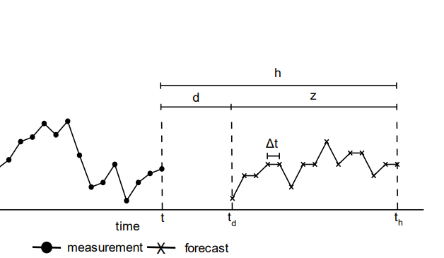
Forecasting terms

• h: Forecasting horizon (how far ahead the forecast looks)

• d: Forecasting delay

• z: Forecasting period (total time covered)

• Δt: Temporal resolution (time between forecast points)

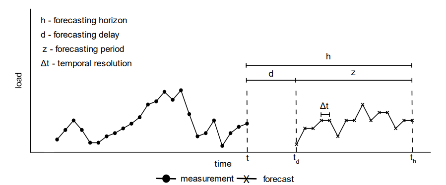
The forecasting horizon

The forecasting horizon is the future time period for which a forecast is generated. For instance, if forecasting the next 100 seconds into the future, the forecasting horizon is 100 seconds.

Target preparation for forecasting

• The electric load column is shifted forward by the forecasting horizon.

• The shifted values become the target for supervised learning.

• The original load remains as an input feature.

Temporal features

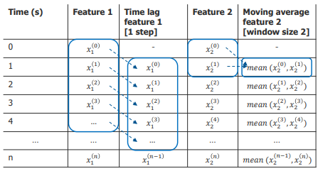
Temporal features are features that capture the time related dependencies in a time series model. Examples for temporal features in forecasting tasks are time lag features and moving average features.

• Time lag features: Add values from previous time steps (e.g., 1 step before load).

• Moving average features: Add averages over a given window size (e.g., last 2 measurements).

• Helps the model learn from historical patterns.

• Time shifts cause some rows to be removed (due to missing values).

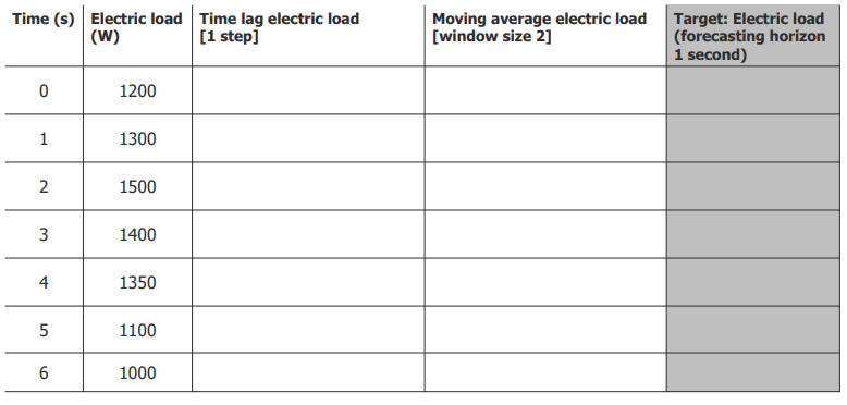
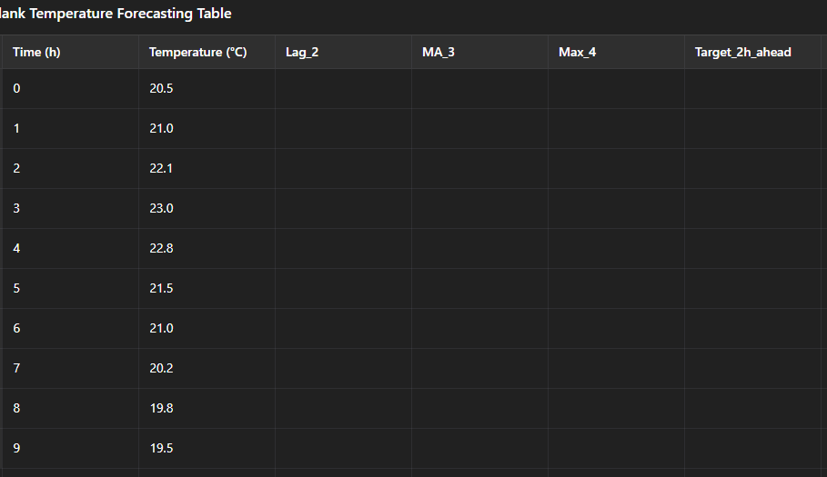
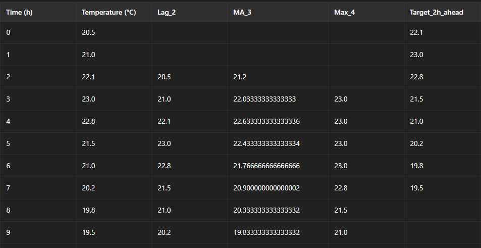
5 minute exercise in small groups: Please fill out the table

1. Time lag electric load [1 step]

   • Take the electric load from the previous time step.

   • For example, at Time = 1, this column takes the value from Time = 0 (1200 W).

   • The first row is empty (NaN) because there is no earlier data.

2. Moving average electric load [window size 2]

   • For each row, calculate the average of the current and previous electric load (window size = 2).

   • For example, at Time = 2, average = (1500 + 1300) / 2 = 1400 W.

   • The first row is empty (NaN) because there isn’t enough data to fill the window.

3. Target: Electric load (forecasting horizon 1 second)

   • Take the electric load value 1 second ahead (forecasting horizon = 1).

   • For example, at Time = 0, target = value at Time = 1 (1300 W).

   • The last row is empty (NaN) because there’s no future data to look at.

Autocorrelation

Autocorrelation is the correlation of a signal with a time lagged copy of itself as a function of time lag.

ACF, bir sinyalin kendisinin zaman kaydırılmış kopyasıyla olan korelasyonunu ölçer.

The autocorrelation function of features helps identifying promising time lags for feature engineering

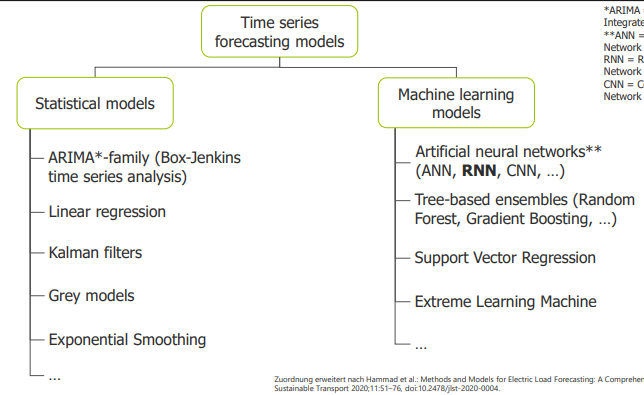
Time series forecasting models

RNN (Recurrent Neural Network)

• Suitable for sequential data (time series, NLP, etc.).

• Different from feedforward networks because of self-loops, letting the hidden state influence the next step.

• During backpropagation, same weight matrices are multiplied repeatedly:

  • Whh<1W_{hh} < 1Whh​<1 → vanishing gradient

  • Whh>1W_{hh} > 1Whh​>1 → exploding gradient

• Solution: Long Short-Term Memory (LSTM) architectures.

LSTM (Long Short-Term Memory)

An improved version of RNN with input (i), forget (f), and output (o) gates to control gradient flow.

• Equations decide what to keep, forget, or output.

GRU (Gated Recurrent Unit)

• Simplified version of LSTM; no separate cell state, only hidden state.

• Controls information with reset gate (r) and update gate (z).

• Fewer parameters → can work with less data but might be less powerful than LSTM.

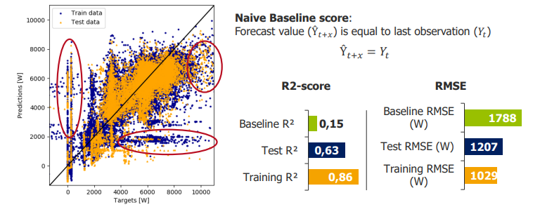
Interpret?

• R²: Baseline (0.15) → Test (0.63) → Train (0.86) → some overfitting.

• RMSE: Test (1207 W) → Train (1029 W) → better than baseline (1788 W).

• Peaks and base load predictions are weaker.

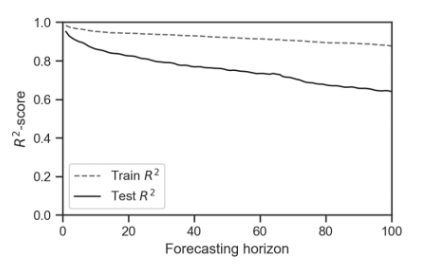
The forecasting accuracy decreases with increasing forecasting horizon

• The graph shows that as the forecasting horizon increases, the R² score decreases.

• Short-term forecasts are more accurate, while long-term forecasts lose accuracy.

• This decline is seen for both training and test sets, with the test curve starting lower.