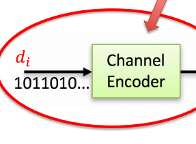
EELE 445 Final

EELE 445 final

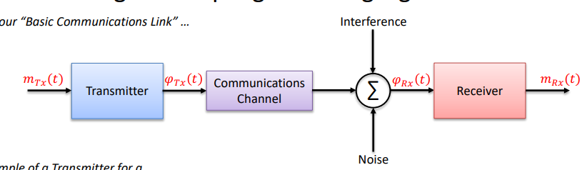
Basic Communications link

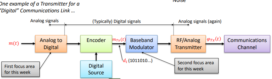
Digital Communications link

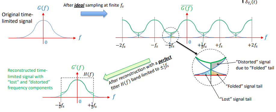
Ideal Sampler

In the real world, all signals are “time-limited” (i.e. not infinite duration) in some regard. Thus, such signals have infinite “tails” in the frequency domain even if at very low amplitude. Such “tails” beyond +-f(s) will get folded back in to the sampled frequency spectrum as shown below:

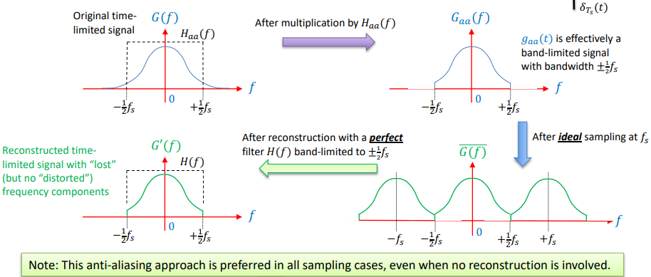
Anti-Aliasing Filter

Thus, for a given finite f(s) used to sample a time-limited signal g(t), we get a better sampled result, whether for reconstruction or otherwise, by applying an “anti-aliasing filter” of bandwidth ± f(s) as illustrated here:

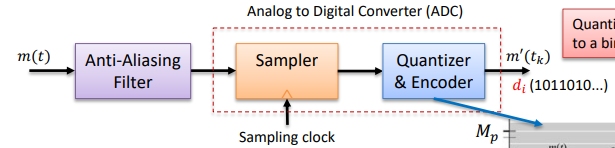
Analog to digital converter

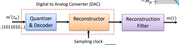
Digital to analog converter

signal-to-(quantization) noise ratio

SNR(Q)

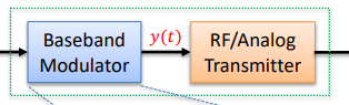
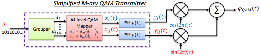
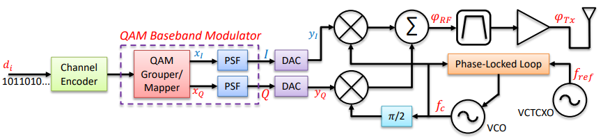
Digital Communications Transmitter

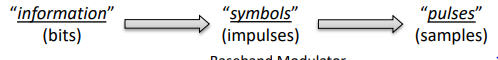
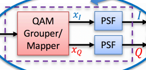
Baseband Modulator

Basic properties of Baseband Modulators

Binary Amplitude Shift Keying

BASK is a simple digital system that is analogous to Broadcast AM Radio.

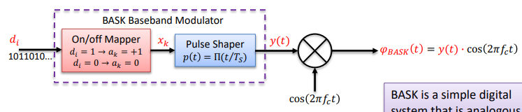
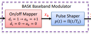
BASK baseband Modulator

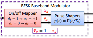
Binary Frequency Shift Keying

BFSK is a simple digital system that is analogous to FM radio, but shown here as complementary BASK modulators. Usually, we implement BFSK using direct modulation of a VCO.

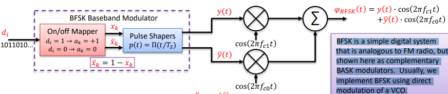
BFSK Baseband Modulator

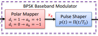
Binary Phase Shift Keying

BPSK Note that we are implementing this “Phase Shift” modulation entirely by changes in amplitude. This modulation is also (correctly) called “2PAM” for “2-level pulse amplitude modulation”

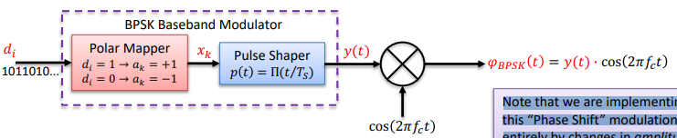
BPSK Baseband Modulator

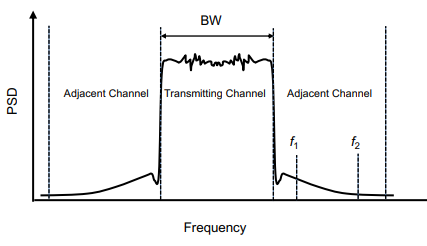
Channel Bandwidth in wireless systems

In wireless systems, the “channel bandwidth” that matters most is the delineation between the transmit channel and the adjacent channels that other transmitters will be using in the same area

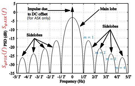
Channel Bandwidth for Rectangular Pulse Shaping ASK/PSK

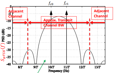
Channel Bandwidth for Rectangular Pulse Shaping FSK

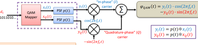
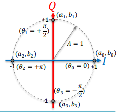
Digital Quadrature Amplitude Modulation

QAM. For analog AM, we saw in Week 2 a doubling of bandwidth in the upconversion process that can be mitigated in terms of bandwidth efficiency by doing single-sideband (SSB) modulation. But there’s another way to get back this factor of 2 in bandwidth efficiency – just modulate two independent carriers at the same frequency but pi/2 apart in phase as depicted below:

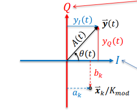
I

In-phase

Q

Quadrature-phase

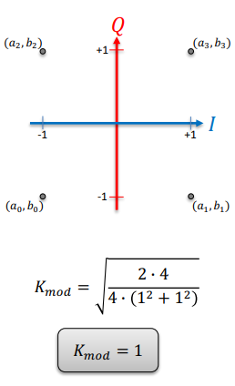
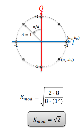
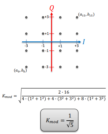
K(mod)

K(mod) is a “normalization” factor for a particular QAM constellation

Single space or constellation Diagram

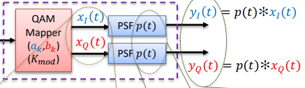
PSF

Pulse Shaping Filter

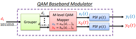
QAM Baseband Modulator

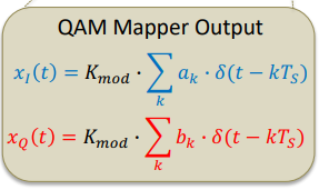
QAM Mapper Output

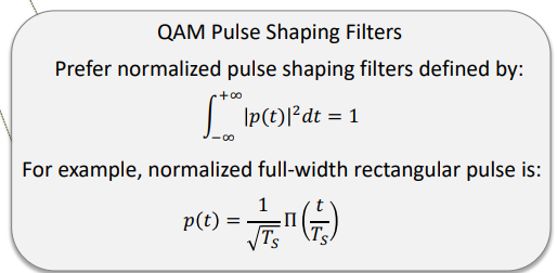
QAM Pulse Shaping Filters

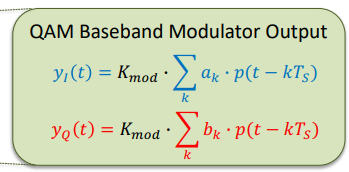
QAM Baseband Modulator Output

binary signaling

In binary signaling, for every bit d(i) to be transmitted, there is a symbol k where a mapper output x(k)(vector) has one value if d(i) = 1 and another value if d(i) = 0.

M-ary signaling

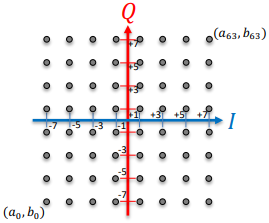
In M-ary signaling, for every consecutive, non-overlapping “group” of “N” bits in the “k-th” set of {d(i), d(i+1),…,d(i+N-1)}(k) to be transmitted, there is a symbol k where x(k)(vector) = k(mod)(a(k)+jb(k)) has one of M values corresponding uniquely to each possible set of N bits, with N = log2(M).

M-level Encoder

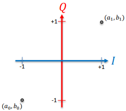
2QAM

Note: “2QAM” is identical to “BPSK”, “2PSK” or “2PAM”. N = log2(2) = 1 bit/symbol

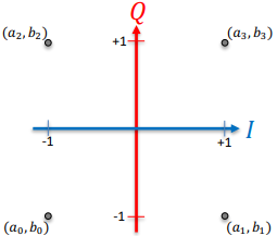
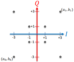
4QAM

Note: “4QAM” is identical to “QPSK” or “4PSK”. N = log2(4) = 2 bits/symbol

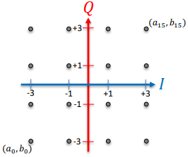
16QAM

Note: This shows “square” 16QAM, but other “shapes” are possible. N = log2(16) = 4 bits/symbol

64QAM

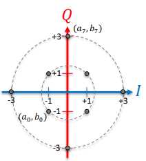
diagonal 8QAM

circular 8QAM

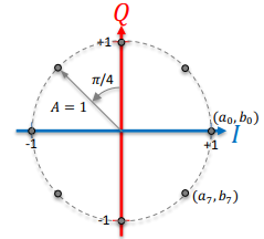
M-ary Digital PSK

Although wireless engineers can describe “Phase Shift Keying” (PSK) via the carrier wave equation, Tx(t) = A(t) * cos[2pif(c )t + theta(t)] where theta(t) is varied as a function of one or more digital bits, in practice MPSK for M ≥ 4 is almost always implemented as an MQAM system with (a(m), b(m)) restricted to constant amplitude A(m) = A for all m and (a(m), b(m)) chosen to describe each theta(m).

M=2 (BPSK)

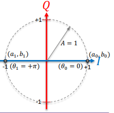
M=4 (QPSK)

M=8 (8PSK)

M-ary QAM Transmitter

4QAM normalization

8PSK normalization

16QAM normalization

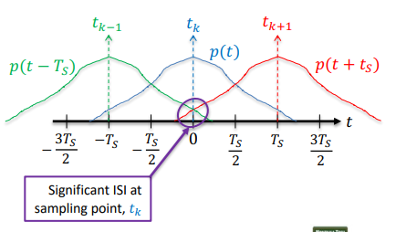
Intersymbol Interference (ISI)

When a pulse p(t) has a non-zero response that overlaps with the non-zero response of subsequent pulses, p(t+nT(s)) , then such pulses “interfere” with each other in a process known as “ISI”, as shown below

Nyquists Criterion for Zero ISI

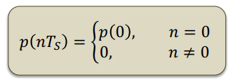
Zero ISI Pulse

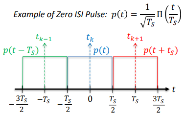
Beta

roll off or excess bandwidth

QAM Transmitter Block Diagram

QAM Transmitter Impairments - Bit domain operations

In the digital bit domain section of a QAM transmitter, there are usually no impairments caused to the system, other than a usually tolerable addition of processing latency. In fact, the purpose of this section is to add controlled amounts of redundancy that can be used at the receiver to overcome “burst” impairments in the overall system, as we will discuss in detail later in this course.

QAM Transmitter Impairments – Baseband Modulator

Grouper/mapper does not cause impairments. Pulse shaping filters create minor impairments due to using finite precision DACs, keeping the filter latency tolerable, and accepting some inter-symbol interference (ISI) at the transmitter to simplify receiver design. This section can also add digital pre-distortion to x(I) and/or x(Q) to compensate for systematic RF impairments

Pulse Shaping Filters for QAM Transmitters

i) Full-width rectangular pulse ii) Root-raised cosine pulse

Properties of Raised Cosine Pulse Shaping Filters

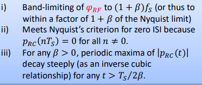
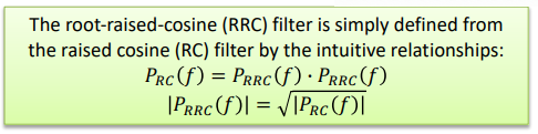
Root Raised Cosine (RRC) Pulse Shaping Filters

why do we use RRC instead of RC?

We need to limit the bandwidth of the transmitter close to Nyquist for efficiency. We also need to band limit in the receiver to set the “noise bandwidth”, and we need to replicate the transmit PSF at the receiver in order to implement an “optimum” receiver. We must meet Nyquist’s criterion for zero ISI at the receiver. Thus, our compromise strategy is to use an RRC baseband filter in both transmit and receive, and the convolution of them both results in an RC filter with zero ISI.

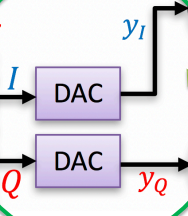
QAM Transmitter Impairments – Digital to Analog Converters

Two significant impairments, both of which we considered and analyzed in Week 3. 1) Finite precision in number of bits (or levels) creates a “quantization noise floor” for y(I) and y(Q). 2) Finite sampling rate ratio to symbol rate causes aliasing in the frequency domain of y(I) and y(Q), but this can be compensated adequately by analog low pass filters not shown above

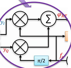
QAM Transmitter Impairments – Vector Modulator (Quadrature Upconverter)

Multiple significant impairments, but only one of consequence for purposes of this course, as others can be compensated. 1) Output noise floor within �(RF), this cannot be compensated for. 2) Mismatch in mixer conversion gains, can be compensated. 3) Phase error in pi/2 phase shifter, can be compensated. 4) Carrier feedthrough in mixers, can be compensated.

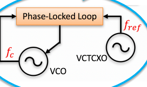
QAM Transmitter Impairments – Local Oscillator (LO) Synthesizer

Multiple significant impairments, but only one of consequence for purposes of this course. 1) Output noise floor of f(c ), usually small compared to output noise floor of �(RF), and thus usually negligible. 2) Drift of f(ref), can be compensated, usually at the receiver. 3) Spurious harmonics of of f(ref), negligible if well designed. 4) Phase noise of f(c ), major problem for 64QAM and above, though can be partially compensated for at receiver.

QAM Transmitter Impairments – Band-select Filter, Power Amplifier (PA) and Antenna

Filter and antenna do not cause significant impairments to the transmitted QAM signal but the PA causes: 1) Non-linear distortion within the transmit channel, thereby causing errors to the modulation domain constellation points and trajectories of �(Tx) that are in excess of any errors already present in �(RF). 2) Intermodulation products in adjacent channels, thereby causing “spectral” re-growth in the frequency domain for the sidebands previously removed by the pulse shaping filters.

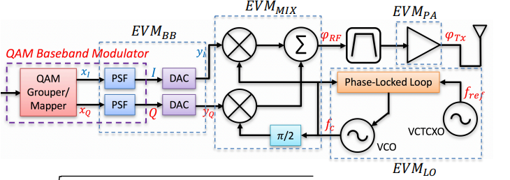
EVM

Error Vector Magnitude

Simplified EVM Model for a QAM Transmitter

Effect of PA Compression on a QAM Transmitter

Power amplifier compression causes a systematic, as opposed to random, error shown as Δ�(PA), wherein the peak amplitude constellation points get reduced in amplitude more than other points.

PAPR

Peak-to-Average Power ratio

ACPR

Adjacent Channel Power Ratio

ACP

Adjacent Channel Power

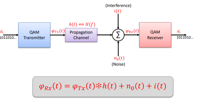
Digital QAM Transmit/Receive RF System

QAM RF Receiver

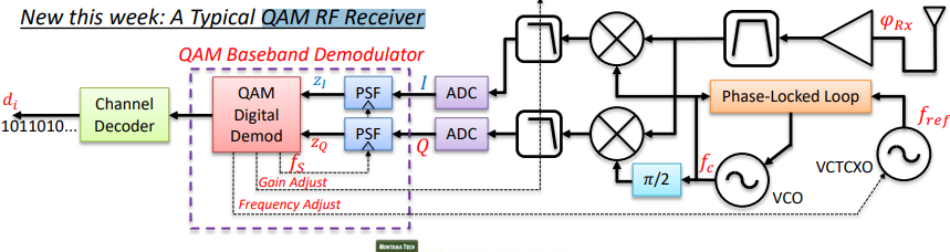
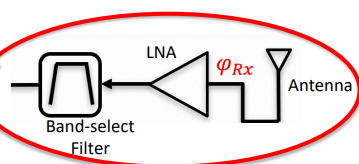
QAM Receiver Functionality – RF Front-End Band-select Filter, Low-Noise Amplifier (LNA) and Antenna

1) The antenna is a transducer that converts radiated electromagnetic energy from the propagation channel into conducted electromagnetic energy in the form of the signal �(Rx). 2) The low-noise amplifier (LNA) linearly amplifies �(Rx) by a power gain, G(LNA), with a relatively small “noise figure”, NF(LNA), such that the overall system noise figure, NF(Rx), is minimized. 3) The band-select filter passes intended baseband channels within �(Rx) but significantly attenuates other signals that may be present in (Rx) from out of band interference.

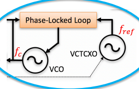
QAM Receiver Functionality – Local Oscillator (LO) Synthesizer

1) The QAM receiver is physically-separate from the remote QAM transmitter, and thus even though this LO synthesizer appears similar to that of the transmitter, there are important consequences from this physical separation. 2) At least because the VCTCXO reference oscillator in the receiver is physically separate from that of the transmitter, then prior to adjustment f(ref(Rx)) is different than f(ref(Tx)). 3) Thus, the synthesized LO at the receiver also differs from that of the transmitter by at least some arbitrary frequency offset Δf(Rx) and some arbitrary phase offset Δtheta(Rx).

QAM Receiver Functionality – Vector Demodulator (aka “Quadrature Downconverter”)

1) Effectively, these downconverting mixers driven by “cos” and “-sin” will “undo” the complex multiply by e^(j2pif(c )t) of the complex low-pass signal y(t)(vector) in the vector modulator of the QAM transmitter. 2) In the time domain, the vector demodulator performs a complex multiplication of a scaled version of the real input signal �(Rx) to generate a complex baseband receive signal. 3) This complex multiplication is most compactly written in the form: e^(-j[2pif(c )t+2pideltaf(Rx)t+deltatheta(Rx)])

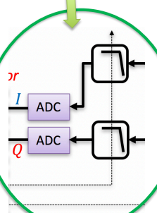
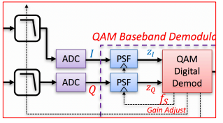
QAM Receiver Functionality – Baseband Analog Baseband Low-Pass Filters, Variable Gain Amplifiers and Analog to Digital Converters

1) The low-pass filters (LPFs) provide rejection of the unwanted vector demodulator frequency components and any undesired signals not within the desired frequency channel for �(Rx), as well as anti-aliasing for the ADCs, with a frequency domain response defined by G(bb(f). 2) The variable gain amplifiers (VGAs), not shown but implied by the dashed arrow through the LPFs, allow the input voltage level into the ADCs to be set. The gain of the VGAs and frequency response of the LPFs together with the gain of the LNA, the mixers, can be collectively modeled within the amplitude scaling of G(bb(f). 3) The ADCs are typically driven by a multiple of f(s).

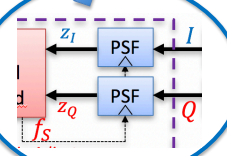
QAM Receiver Functionality – Matched Filters

) Textbooks prove that an optimal digital receiver has “filters” that exactly “match” the transmitter. 2) Here we skip the derivation and simply jump to the intuitive end result – that the receive matched filters are mirrored replicas of the transmit PSFs (p(−t) ⟺ p(−f)), except that to obtain complex impulse outputs, z(l)(vector), then the output of the receive PSFs are sampled at a time t(l) derived from the symbol (or sample) clock with frequency f(s). 3) When the receive sample clock nominally equals the transmit symbol clock, then: t(l) = T(0)+l*T(s) where T(0), is the receiver symbol timing offset (STO) that aligns the impulses z(l)(vector) at the receiver to the impulses x(k)(vector) as referred to the transmitter.

STO

symbol timing offset

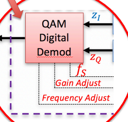
QAM Receiver Functionality – QAM Digital Demod

1) The QAM Digital Demod functionality operates in two fundamental modes: the first mode involves adjustment and training from a series of known “reference” symbols in a “header” or “preamble”, and the second mode involves actual demodulation of unknown “payload” symbols. 2) At a minimum, the first mode requires performing automatic gain control (AGC), carrier frequency offset (CFO) adjustment, symbol timing offset (STO) adjustment, carrier phase offset (CPO) adjustment and channel estimation. 3) At a minimum, the second mode requires performing channel equalization based upon the channel estimate as well as the “inverse” operations to those of the QAM Grouper/Mapper in the transmitter.

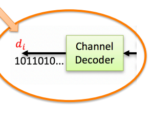
QAM Receiver Functionality – Bit Domain

1) Most modern QAM systems use channel encoding with forward error correction (FEC) to overcome “burst” errors, whether due to noise or other impairments. 2) Typically, channel encoding and decoding also includes interleaving and de-interleaving across large blocks of coded bits. 3) In many modern systems, this Channel Decoder (and De-Interleaver) functionality operates iteratively in combination with the QAM Digital Demod functionality

FEC

Forward Error Correction

QAM Receiver Synchronization using known preambles

In order to enable a receiver to synchronize with a transmitter, most digital wireless systems transmit known patterns often called “preambles”. In cellular systems, these known patterns are often sent at known points in time. In Wi-Fi systems, these known patterns are usually sent at the beginning of every “packet” or “frame” transmission

QAM Receiver Preamble Processing, Step 1: AGC

In Step 1, the QAM Digital Demod computes |z(l)(vector)| from all available samples, whether l has been optimized for STO or otherwise, to at least adjust the analog gain as indicated by the low pass filters in our generic receiver block diagram such that the “full scale” input to the ADCs is not exceeded.

Eventually the AGC process, whether entirely by analog gain control or by some mix of analog gain control and linear digital sample scaling, must eventually converge at |z(l)(vector)| = |x(k)(vector)| at least for the known symbols, x(k)(vector), within the preamble sequence. This corresponds to applying a correction factor of 1⁄A(TR)such that A’(TR) = 1 after the synchronization process has converged.

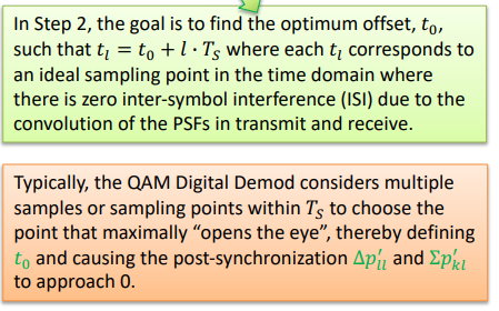
QAM Receiver Preamble Processing, Step 2: STO

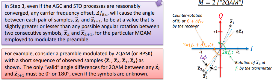
QAM Receiver Preamble Processing, Step 3: CFO

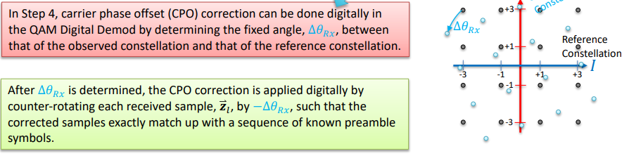
QAM Receiver Preamble Processing, Step 4: CPO

CPO

Carrier Phase Offset

n(o)(t)

noise

i(t)

Interference

Interference

Any undesired signal that is received at the receiver input transducer. For an RF wireless system this means any undesired radiated emission that reaches the receiver antenna. Interference is typically deterministic at its source even if unknown and “random” at the receiver.

Noise

At the receiver input transducer, such as an antenna for an RF wireless system, “noise” means the random signal fluctuations that are generated by the real impedance of the input transducer. Noise is not deterministic. It is “Gaussian”.

Random Thermal noise

Any electrical conductor will generate “thermal noise” that is frequency independent (to the extent the real impedance is frequency independent ) with a uniformly random phase (or sign) and a “normal” or Gaussian amplitude distribution.

SER

Symbol Error Rate

SNR

signal to noise ratio

BER

Bit Error Rate

SER versus BER

BLER

Block Error Rate

FER

Frame error rate

PER

Packer error rate

Block/Frame/Packet Error Rate versus Symbol Error Rate

f(s)

symbol rate

R(d)

data transfer rate

Two Major Types of Co-channel Interference

1) Interferer’s f(c ) is same as the receiver. 2) Interferer’s ACP falls within receive channel.