Chapter 10: How to make predictions with a linear regression model

Unlike a simple linear regression model, a multiple regression model:

a. has two or more dependent variables

b. results in a curved line when the relationships are plotted

c. results in a straight line when the relationships are plotted

d. has two or more independent variables

d. has two or more independent variables

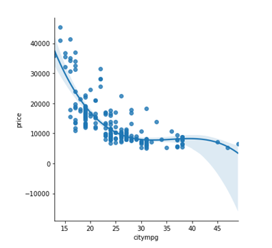
Refer to the Seaborn Regression plot. This code creates the regression plot:

a. sns.lmplot(data=carsData, x='citympg', y='price', logistic=True)

b. sns.lmplot(data=carsData, x='citympg', y='price', order=3)

c. sns.lmplot(data=carsData, x='citympg', y='price', poly=True)

d. sns.relplot(data=carsData, x='citympg', y='price', kind='regression', scatter=True)

b. sns.lmplot(data=carsData, x='citympg', y='price', order=3)

This code creates a linear regression model:

a. model = LinearRegression()

model.train(x_train, y_train)

b. model = LinearRegression(x_train, y_train)

c. model = LinearRegression()

model.train(x_train, x_test)

d. model = LinearRegression()

model.fit(x_train, y_train)

d. model = LinearRegression()

model.fit(x_train, y_train)

The four steps in the procedure for creating and using a regession model are:

a. train_test_split(), score(), fit(), predict()

b. train_test_split(), predict(), fit(), score()

c. train_test_split(), fit(), predict(), score()

d. train_test_split(), fit(), score(), predict()

d. train_test_split(), fit(), score(), predict()

A simple linear regression model is used to predict the value of:

a. one independent variable based on the values of one dependent variable

b. one dependent variable based on the values of two or more independent variables

c. one dependent variable based on the values of one independent variable

d. one independent variable based on the values of two or more dependent variables

c. one dependent variable based on the values of one independent variable

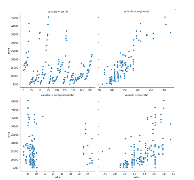
Based on the following scatter plots, which variable has the best correlation with price?

a. enginesize

b. car_ID

c. boreratio

d. compressionratio

a. enginesize

This code creates a DataFrame of predicted values:

a. y_predicted = model.predict(x_test).to_frame()

b. y_predicted = model.predict(x_test)

c. y_predicted = model.predict(x_test)

pd.DataFrame(y_predicted, columns=['predicted'])

d. y_predicted = model.score(x_test)

pd.DataFrame(y_predicted, columns=['predicted'])

c. y_predicted = model.predict(x_test)

pd.DataFrame(y_predicted, columns=['predicted'])

The corr() method generated the following r-values. Which one is the strongest?

a. 0.72

b. -0.84

c. 0.46

d. -0.23

b. -0.84

Refer to the predictions DataFrame. This code adds the residuals to the DataFrame:

a. predictions[['residuals']] = predictions.price - predictions.predictedPrice

b. predictions[['residuals']] = predictions.residuals('price', 'predictedPrice')

c. predictions[['residuals']] = model.residuals()

d. predictions[['residuals']] = predictions.predictedPrice - predictions.price

a. predictions[['residuals']] = predictions.price - predictions.predictedPrice

Refer to the Seaborn Regression plot. This code plots the residuals for this regression plot:

a. sns.residplot(data=carsData, x='citympg', y='price')

b. sns.relplot(data=carsData, x='citympg', y='price', kind='line',

c. sns.residplot(data=carsData, x='citympg', y='price', poly=True)

d. sns.residplot(data=carsData, x='citympg', y='price', order=3)

d. sns.residplot(data=carsData, x='citympg', y='price', order=3)

Two common ways to identfy the correlations between variables are:

a. line plots and the corr() method

b. line plots and the corr_vars() method

c. scatter plots and the corr() method

d. scatter plots and corr_vars() method

c. scatter plots and the corr() method

Refer to the residuals DataFrame. This code plots the residuals:

a. g = sns.relplot(data=residuals, x='enginesize', y='residuals',

kind='scatter')

for ax in g.axes.flat:

ax.axhline(0, ls='--')

b. g = sns.relplot(data=residuals, x='enginesize', y='residuals')

for ax in g.axes.flat:

ax.axhline(0, ls='--')

c. g = sns.residplot(data=residuals, x='enginesize', y='residuals')

for ax in g.axes.flat:

ax.axhline(0, ls='--')

a. g = sns.relplot(data=residuals, x='enginesize', y='residuals',

kind='scatter')

for ax in g.axes.flat:

ax.axhline(0, ls='--')

The regression residuals show

a. the average difference between the actual values and the predicted values

b. the differences between the actual values and the predicted values

c. the strength of the correlations between the independent variables and the dependent variable

d. the percent of the variation in the dependent variable that can be explained by the independent variable

b. the differences between the actual values and the predicted values