Probability theory, confidence intervals, t-distribution

Topic 5

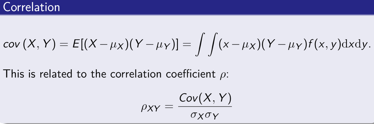
Covariance

Measure of correlation between two random variables - related to correlation coefficient

A positive covariance typically indicates that as one variable increases so does the other

Related to the correlation coefficient

Probability theory - properties of the expected value

E(a) = a

E(aX) = aE(X)

E(aX + b) = aE(x) + b

E(X + Y) = E(X) + E(Y)

E(X) = \muX

Unless X AND Y are independent E(XY) \ne E(X)E(Y)

Probability theory - properties of the Variance

var(X) = E[(X - \mu x)²]

var(b) = 0

var(X + b) = var(X)

var(aX + b) = a²var(X)

var(X + Y) = E[(X + Y - E(X) - E(Y))²] = var(X) + var(Y) + 2cov(X, Y)

var(aX + bY) = a²var(X) + b²var(Y) + 2abcov(X, Y)

cob(X, X) = var(X)

What makes a good estimator

Must be unbiased, efficient and consistent

Used for inferential stats e.g. determine the mean income of UK residents and use an estimator to estimate the population value for mean income

Unbiased estimator

Statistical estimator whose expected value is equal to the true value of the parameter being estimated

We know from the Central Limit theorem that the sample mean is an UNBIASED estimator of the population mean because its sampling distribution is centred on the population mean

Efficient estimator

Less dispersed - lower variance and lower standard deviation, and more accurate estimators are more efficient

Can also improve efficiency by increasing the size of the sample used

Unbiased and efficiency estimator trade-off

• Unbiased and efficient estimator gives us the best chance of getting an estimate close to the true value

• Biased but efficient estimator would provide estimates that are clustered but around the wrong value

• Unbiased and inefficient estimator estimates the true value but in practice the chances of the estimate being close to the true value are low

• Biased and inefficient estimator we wouldn’t even get close on average let alone with a single sample to the true value

Point estimate

The statistic computed from sample information that estimates a population parameter e.g. sample mean x bar is the point estimate of the population mean mew

Confidence intervals

Range of values constructed from sample data so that the population parameter is likely to occur within that range at a specified probability (known as the confidence level)

CI = point estimate ± margin of error

Confidence interval for population mean with known standard deviation - formula general

\overline{x}\pm z_{\alpha}\frac{\sigma}{\sqrt{n}}

e.g. 95% confidence interval - asking what values of z would there be 95% of the area under the standard normal distribution curve -

z value from table is 1.96

so interval -1.96 to 1.96 - using formula

\overline{x}\pm1.96\frac{\sigma}{\sqrt{n}}

and you should have values for sample mean, s.d. and sample size - TO PLUG IN

Steps to calculate a Confidence Interval

Choose level of risk you’re comfortable with - interval estimate needs to include\mu

Probability of this error is alpha - usually alpha = 0.05/95% confidence

Find z score for chosen confidence level

Plug values into CI general formula - and the confidence intervals will then have a lower and upper bound

Interpret results

e.g. answer = 35,000 ±175.31 - for question about population’s mean income

so we are 95% confident the pop mean income lies between £34,825 and £35,175

(as n increases the confidence interval range get smaller - so bigger sample better as more informative as to what the true mean might be)

Confidence Interval when standard deviation unknown

Use the ‘t-statistic’

t=\frac{\left(\overline{x}-\mu\right)}{\frac{s}{\sqrt{n}}}-t_{n-1}

The CI is

\overline{x}\pm t_{\alpha,n-1}\frac{s}{\sqrt{n}}

s replaces \sigma - in new formula (but is still s.d.)

The t statistic value for 95% confidence is 1.96 - same as standard normal

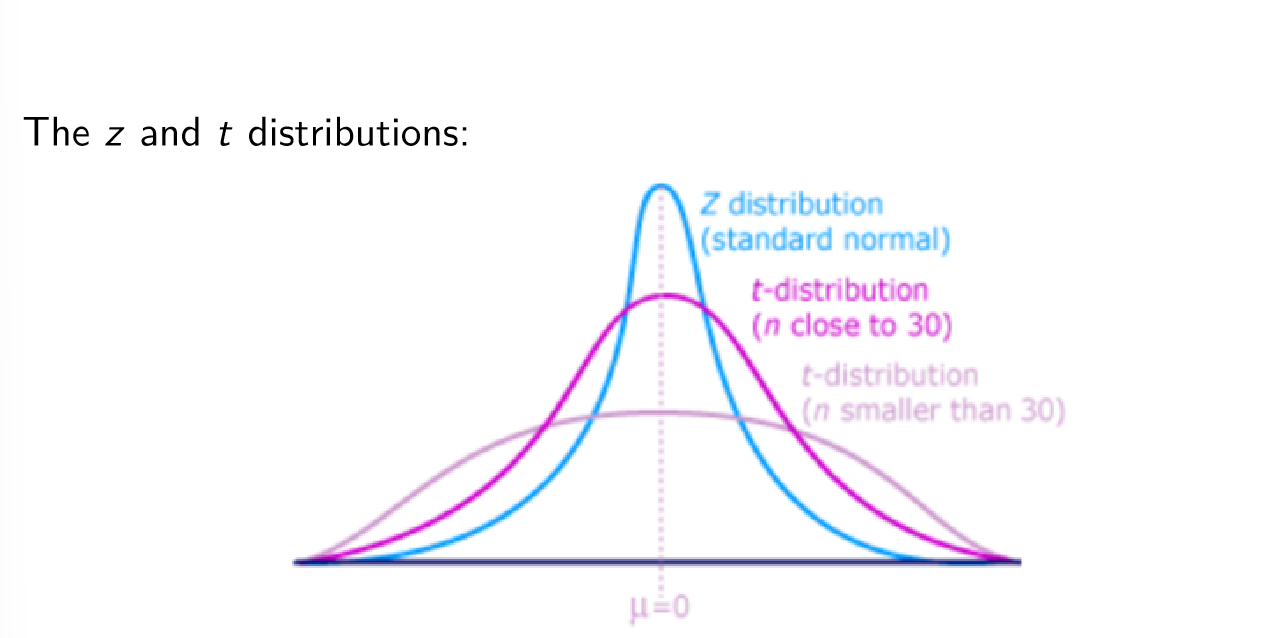
t distribution

Similar to standard normal distribution: continuous, bell shaped, mean (mew) = 0, BUT more spread out and flatter at centre than standard normal - as n increases t distribution approaches standard normal

There are a family of t distributions - all have mean of 0 but their s.d. differ according to the sample size

n-1 = distribution’s degrees of freedom (d.f.)

More spread out than z so confidence intervals will be wider for the same level of confidence

Confidence Interval when s.d. unknown

Use n = sample size

x bar = sample mean

s = s.d.

Use table to find n-1 degrees of freedom critical value

Then use t distribution formula and plug in n, xbar, s values AND critical value into t_{\alpha,n-1} section

Will get upper and lower bound numbers - found confidence interval

How to choose confidence level

Typically use

\alpha = 0.01 (99% confidence), 0.05 (0.95% confidence) and 0.1 (90% confidence)

Confidence interval for a population proportion

Sample proportion formula: p = x/n where x is the number of ‘successes’, and n is the sample size

The values n \pi and n(1- \pi ) should both be greater than or equal to 5

The situation can be represented by a BINOMIAL distribution

Formula: p\pm z\sqrt{\frac{p\left(1-p\right)}{n}}

Step 1: calculate sample proportion using p = x/n

Step 2: find z value for confidence level e.g. 1.96 for 95% CI

Step 3: Input values to find upper and lower bound values - which gives an estimate for % of a population that counts as a ‘success’ value

What do we mean by a ‘large’ sample size

Use formula:n=\left(\frac{z\sigma}{E}\right)^2 for POPULATION MEAN estimate

where z is the standard normal value corresponding to desired level of confidence

\sigma is the population standard deviation

E is the max allowable error

Use formula: n=\pi\left(1-\pi\right)\left(\frac{z}{E}\right)^2 for POPULATION PROPORTION estimate

where z is the standard normal value corresponding to desired level of confidence

\pi is the population proportion - and if we can’t get a rough idea where the population proportion might be use 0.50

E is the max allowable error

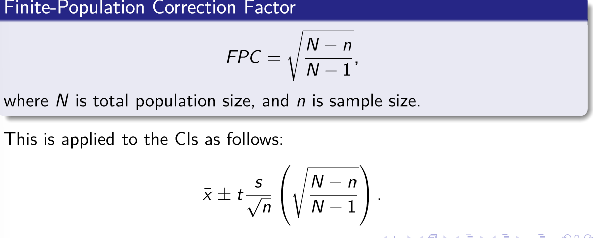
Finite population correction factor

Where N is the total population size and n = sample size