Stats 10 Midterm- UCLA

Variable

any characteristics, number, or quantity that can be measured or counted. It is called a ---- because the value may vary between data units in a population, and may change in value over time or observation. (usually put on columns in data table)

Observation

occurrence of a specific variable that is recorded about a data unit. (usually put on rows in data table)

Population

collection of observations of interest. This number is usually very large and nearly impossible to obtain measurements from.

Sample

portion of a population of interest. A sample is usually taken to measure a characteristic about a population.

Numerical

---- Variable (Quantitative) : Temperature, GPA, Height, Distance, ...

Categorical

---- Variable (Qualitative) : Eye color, Gender, Year in school, Major in college, ...

Frequency

natural way to summarize the categorical variables

Confounding Variable

A difference between the two groups that could explain why the outcomes were different. affects the variables of interest but is not known or acknowledged, and thus (potentially) distorts the resulting data

observational study

In an ---- ---, researchers don't assign choices, they simply observe them

experimental study

In an experiment, the experimenter actively and deliberately manipulates the treatment variable and assigns the subjects to those treatments, generally at random.

Large sample size, Random assignment/ bias, Double-blinded experiment, placebo

Four things that are important in an experimental study:

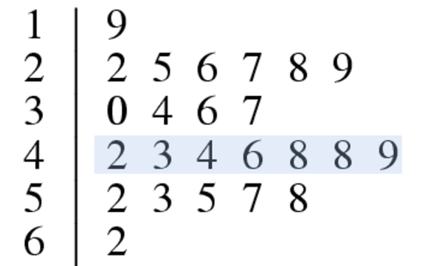
Stem-and-leaf plot

Divides each observation into a "stem" and "leaf". Best for numerical data

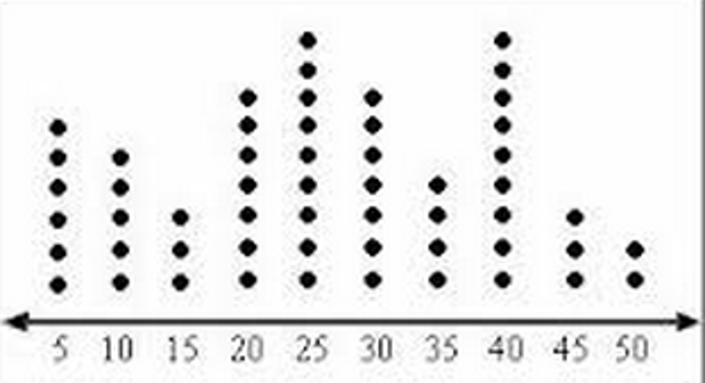
Dot Plot

Places a dot along an axis for each case in the data. Best for numerical data

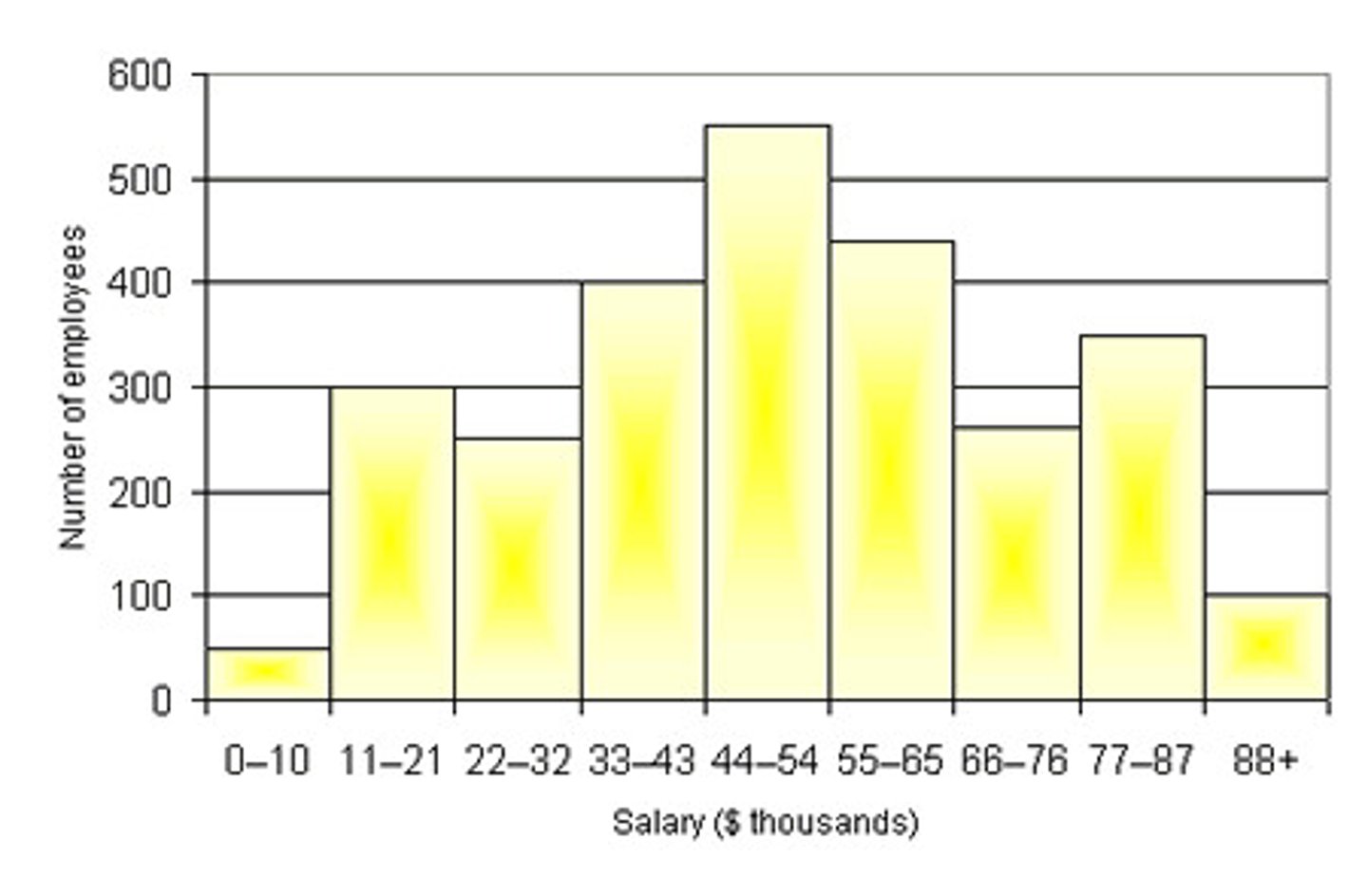
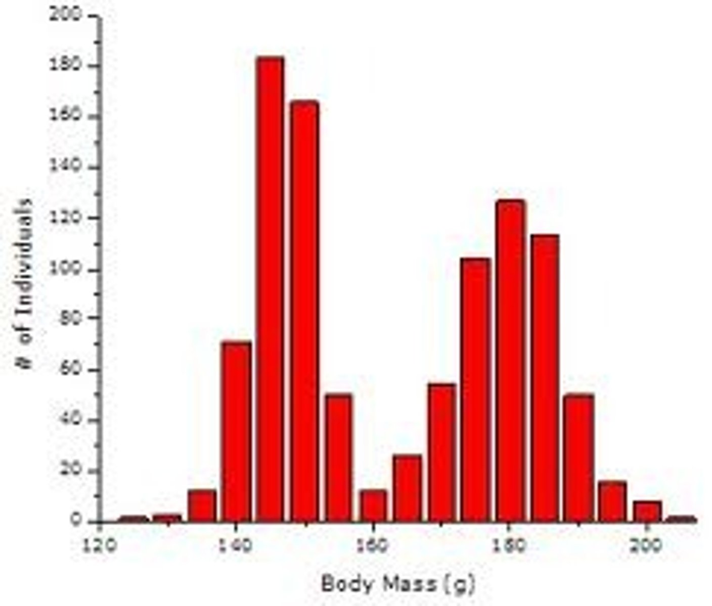
Histogram

displays the number of cases in each bin. (Bin widths are a personal choice. Too small a width shows too much detail while too large a width shows too little.)

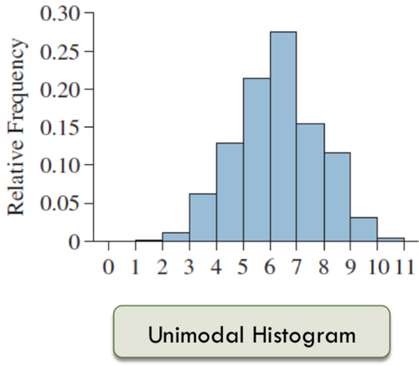
The horizontal axis is numerical and the vertical axis is the (relative) frequency. Best for numerical data

relative frequency

how often something happens divided by all the possible outcomes. Used in histogram y-axis

Shape

focuses on number of modes (peaks), Symmetricity, outliers, central tendency

Unimodal

single mode

Bimodal

two modes

Uniform

no apparent peaks

Symmetric

the left hand side is roughly the mirror image of the right hand side. (bell-shaped)

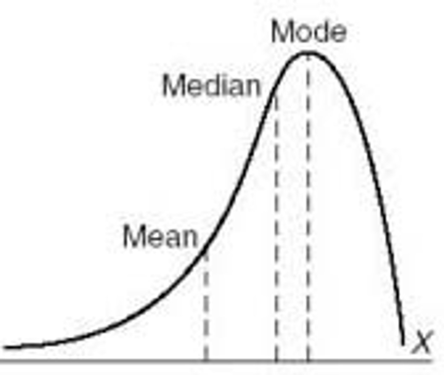
Right-Skewed

(positively skewed) : long tail to the right

Left-Skewed

(negatively skewed) : long tail to the left

Outliers

unusually large or small values in the distribution

typical value

not necessarily center in location. Whether its in the center or not

spread/ variability

how spread out the data is from the center

When the data values are tightly clustered around the center of the distribution, the spread is small

When data values are scattered far from the center, the spread is large

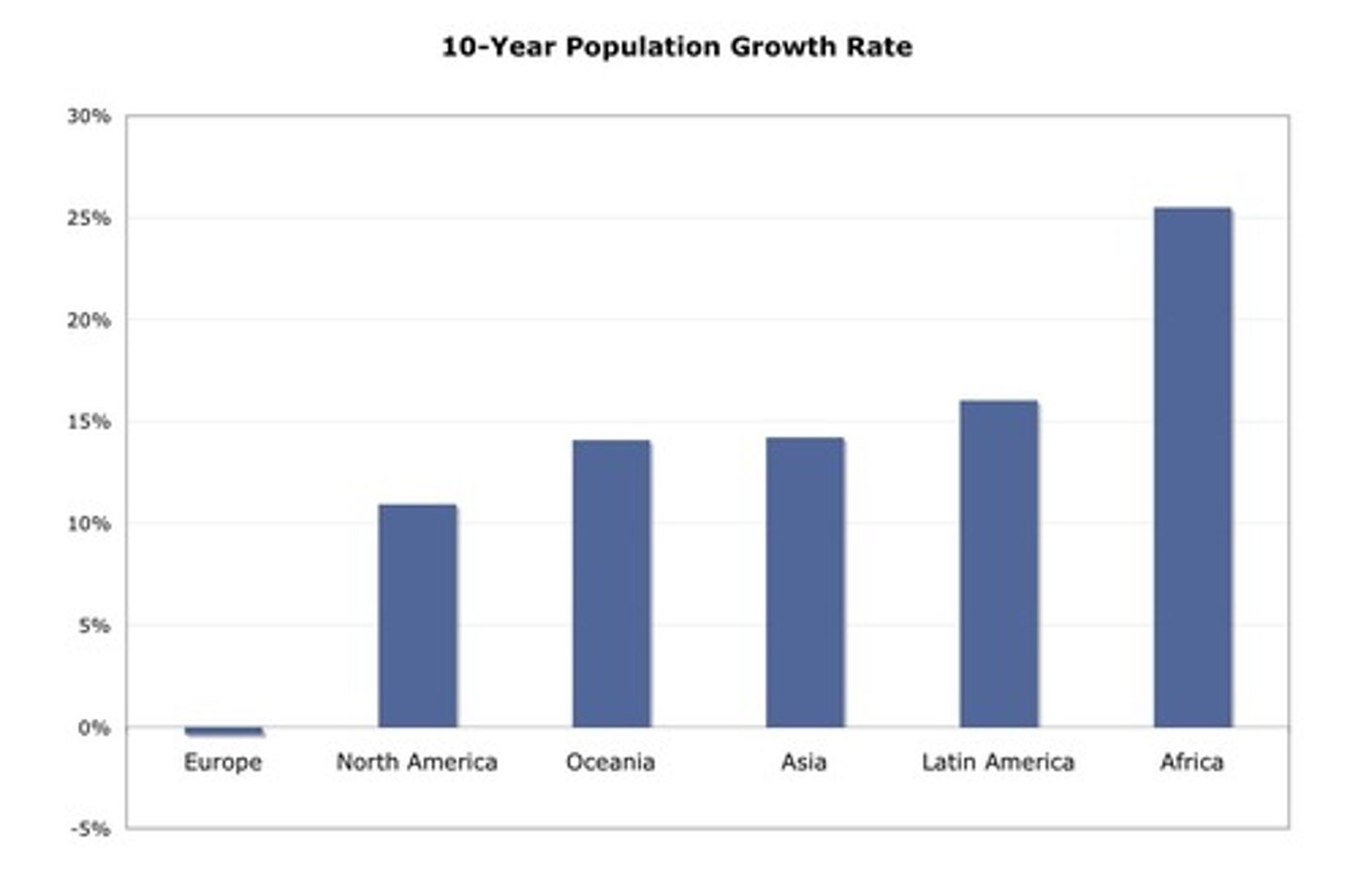
Bar Chart

Displays counts of each category next to each other for easy comparison. May put relative frequency proportions for each category. Best for categorical data

Mean

The center as a balancing point. Arithmetic average (calculation)

standard deviation

The average distance of a value from the mean.

It measures how far away the typical observation is from the mean. In symmetric, unimodal distributions, the majority (more than half) of the observations are less than one ---- from the mean.

Empirical Rule

A rough guideline, a rule of thumb, that helps us understand how the standard deviation measure variability. According to the ----, 68% of the data will fall between 85 and 115 (one SD from the mean), 95% of the data will fall between 70 and 130, and 99.7% of the data will fall between 55 and 145.

z-score

measure the distance of each data value from the mean in standard deviations. A negative --- tells us that the data value is below the mean, while a positive --- tells us that the data value is above the mean.

magnitude

of z-score (absolute z-score) implies the'unusualness' of the observation regardless itsdirection.

median

The center as the middle (half-way point)

IQR

tells us how much space the middle 50% of the data occupy.

scatterplot

are the best way to start observing the relationship and the ideal way to picture associations between two numerical variables.you can see patterns, trends, relationships, and even the occasional extraordinary value sitting apart from the others

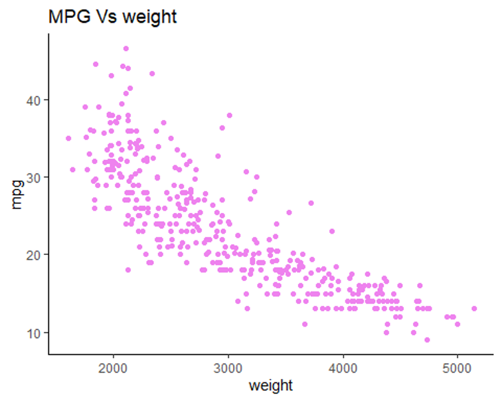
explanatory variable

The variable in the x-axis (aka independent variable)

response variable

the variable on the y-axis is called the (aka dependent variable)

linear

If the points appear as a cloud or swarm of points stretched out in a generally consistent, straight form, the form of the relationship is

correlation coefficient

(r) gives us a numerical measurement of the strength of the linear relationship between the explanatory and response variables. A correlation near zero corresponds to a weak linear association.

regression line

Tool for making predictions about future observed values. Provides us with a useful way of summarizing a linear relationship

predicted value

The estimate made from a linear model. denoted as ^Y

residual

The difference between the observed value and its associated predicted value

line of best fit

the line for which the sum of the squared residuals is smallest. Among possible regression lines, find the line that minimizes the sum or squared residuals.

random

no predictable pattern occurs and no digit is more likely to appear than any other

theoritical probability

the relative frequency at which an event happens after infinitely many repetitions.

trial

Each time you hit shuffle

outcome

The song that plays as a result of hitting shuffle

sample space

the collection of all possible outcomes of a trial

event

A combination of outcomes

independent

the outcome of one trial doesn't influence or change the outcome of another.

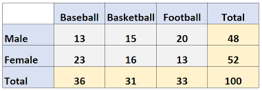
two-way table

displays the count of two categorical variables at a time conditional on each other

Treatment group

people who receive the treatment (or have the characteristic of interest)

Control group

people who do not receive the treatment (or do not have the characteristic of interest)

mode

value of the data set that occurs with the greatest frequency

types of bar charts

pareto (greatest to least), side-by-side, segmented(both display two categorical variables graphically), pie chart

boxplot

useful graphical tool for visualizing a distribution, especially when comparing two or more groups of data, five-number summary

scatterplot three patterns

strength (how closely they’re clustered), direction (positive or negative), and shape (linear or non-linear) 

Correlation vs Causation

a high correlation between two variables does NOT imply causation

Measure of Goodness of fit 

If the correlation between x and y is r = 1, or r = -1, then the model would predict y perfectly, and the residuals would all be 0, hence variability in the response variable would be explained by the explanatory variable 

R² coefficient of determination

gives us the percentage of the variance of y accounted for by the regression model or in other words explained by x

Residual Plot Bad examples 

Fan shaped residuals, Curved residuals 

empirical probability 

relative frequencies based on an experiment or on observations of a real life process

theoretical probability example

we may not be able to predict which song we play each time we hit shuffle, however we know in the long run 5 out of 1000 songs will be JB songs

empirical probability example

we listen to 100 songs on shuffle and 4 ofthem are JB songs, the empirical probability is 4/100 = 0.04

Complement rules

the set of outcomes that are not in the event A is called the complement of A denoted A^c

Complement rule example

A: it rains in LA 0.4

A^c : it does not rain in LA 0.6

Disjoint events (Mutually exclusive event)

Events that have no outcomes in common and thus cannot occur together

Combined events

Event A and B happen at the same time, Event A or B either or both happen

Conditional probability

we focus on one group of objects and imagine taking a random sample from that group alone.

Law of Large Numbers

the long run relative frequency of repeated independent events gets closer and closer to the true relative frequency as the number of trials increases.