ML System Design

Should you use ROC-AUC or PR-AUC with class imbalance?

If your problem has strong class imbalance (e.g. 99% of the data is negative, 1% is positive), PR-AUC is going to be a far better metric than ROC-AUC. ROC-AUC can look fantastic even if the classifier is completely useless for highly imbalanced problems.

What is online evaluation?

For online evaluation, you'll often want to implement a shadow mode test where the model makes predictions but doesn't take action, allowing reviewers to validate results. Once confidence is established, move to an A/B test measuring both technical metrics and business impacts like user retention and reviewer workload.

What is offline evaluation?

For offline evaluation, establish a balanced test set with stratified sampling to ensure adequate representation of all content categories. Use precision-recall curves to find the optimal threshold that maintains your required precision while maximizing recall. The important thing is that your offline evaluation is correlated with the outcomes of your online evaluations!

What are classification systems?

In classification systems, we're taking some input (e.g. an image and some text) and we're predicting some output (e.g. a classification label). Classification systems will often have a labelling component with non-trivial cost, so an important consideration is how resource-efficient you can be in conducting these evaluations. They also frequently "fill in" for humans doing manual work, which provides good baselines for thresholds and clues to the right metrics to use to evaluate.

Example problems: Content moderation, spam detection, fraud detection

Business Objective

For classification systems, the business objective will often be downstream of the classification. Ask yourself "what action is taken as a result of the classification?" and "how does that action impact the business?" For example, in a content moderation system, the primary business goal is minimizing harmful content exposure while avoiding false positives that might frustrate legitimate users. This impacts user retention and operational review costs.

Product Metrics

Product metrics will vary wildly by application, but some common ones include:

• User retention rate

• Time to label (moderate/evaluate/judge/etc)

• User satisfaction scores

• Operational review costs

• Appeal rate for moderation decisions

• Downstream costs associated with errors (both false-positives and false-negatives)

ML Metrics

For measuring classification systems, it's common to use the language of precision and recall. Precision is the percentage of positive predictions that are actually positive. Recall is the percentage of actual positives that the model correctly identifies. Classification performance can often be summarized with a precision-recall curve, which shows the trade-off between precision and recall for different threshold values.

We can tune the threshold arbitrarily according to the business objective: if we care more about precision, or more about recall, we can increase or decrease the threshold. For many applications, fixing precision at some arbitrary threshold — often around human-level performance — is a good way to ensure the system is useful.

Some common metrics include:

• Precision at your operating threshold (e.g., 95%)

• Recall at that precision

• ROC-AUC for binary classification

• F1 score (harmonic mean of precision and recall)

• PR-AUC for overall model quality

• False positive rate for different content segments

• Per-class performance for multi-class classification systems

If your problem has strong class imbalance (e.g. 99% of the data is negative, 1% is positive), PR-AUC is going to be a far better metric than ROC-AUC. ROC-AUC can look fantastic even if the classifier is completely useless for highly imbalanced problems.

Evaluation Methodology

For online evaluation, you'll often want to implement a shadow mode test where the model makes predictions but doesn't take action, allowing reviewers to validate results. Once confidence is established, move to an A/B test measuring both technical metrics and business impacts like user retention and reviewer workload.

For offline evaluation, establish a balanced test set with stratified sampling to ensure adequate representation of all content categories. Use precision-recall curves to find the optimal threshold that maintains your required precision while maximizing recall. The important thing is that your offline evaluation is correlated with the outcomes of your online evaluations!

What are common classification system evaluation challenges?

• Class Imbalance

  • Most real-world classification problems have highly imbalanced class distributions. For example, in fraud detection, legitimate transactions vastly outnumber fraudulent ones. This effects the datasets you assemble for evaluation, and the metrics you choose to evaluate. For highly imbalanced problems, PR-AUC is a far better metric than ROC-AUC. In interviews, you may also want to talk about a loop for discovering previously unseen instances of the minority class.

• Label Efficiency

  • Obtaining high-quality labels is often expensive and time-consuming, especially for specialized domains requiring expert knowledge. Especially in the presence of class imbalance, random sampling is a poor way to acquire labels which will reduce variance in your evaluation metrics. Employing stratified sampling approaches using classifiers scores can be useful, or even using active learning to prioritize labeling the most informative examples.

• Estimating Prevalence

  • In many applications, the true prevalence of positive cases in production may be hard to measure: in most cases you won't know the "right" answer without expending considerable resources (e.g. running a human review), hence the reason for the ML system in the first place. Random sampling is a good, unbiased way to estimate prevalence but suffers from high variance. Imagine you have a problem where <1% of the data is positive: if you randomly sample 100 examples you'll only have 1 positive example to estimate prevalence from.

• Feedback Loops

  • Finally, classification systems can create feedback loops where the model's predictions influence future test data, potentially amplifying biases or errors over time. Some ways to solve this include: regularly inject randomness into the system (e.g. withhold actions you might otherwise take) to explore the full data space, or maintain a golden set of examples unaffected by the model's decisions.

What is the general ML evaluation framework for interviews?

1. Business Objective: We'll start with the business objective. If you're following our delivery framework, the business objective will be top of mind. Working backwards from this objective will ensure your metric is tethered to something real and valuable, not an arbitrary vanity evaluation.

2. Product Metrics: Next we'll work up to the product metrics: explain which user-facing metrics will indicate success. Think about what you can measure in the performance of the product or system which will indicate success.

3. ML metrics: With product metrics in place, we can detail technical metrics that align with the product goals. These should be metrics you can measure in the performance of the ML system, often without requiring new inputs (labels, user feedback, simulation results, etc.)

4. Evaluation Methodology: With our metrics in place, we'll discuss how we can measure them. Outline both online and offline evaluation approaches. Oftentimes your offline evaluations will be a proxy for the online evaluation, but geared towards rapid iteration.

5. Address Challenges: Finally, your evaluation will invariably include some challenges. Imbalanced data, labelling costs, fairness issues, etc. You'll finalize the evaluation discussion by discussing potential pitfalls and how you'd mitigate them.

What are the common classification metrics?

Precision: The percentage of positive predictions that are actually positive.

• Intuition: "When the model says something is harmful content, how often is it right?"

• Calculation: (True Positives) / (True Positives + False Positives)

Recall: The percentage of actual positives that the model correctly identifies.

• Intuition: "What percentage of all harmful content does the model catch?"

• Calculation: (True Positives) / (True Positives + False Negatives)

PR-AUC: Area under the Precision-Recall curve.

• Intuition: "How well does the model balance precision and recall across different thresholds?"

• Ranges from 0 to 1, with higher values being better

F1 Score: The harmonic mean of precision and recall.

• Intuition: "A single number balancing how many positives we catch vs. how accurate our positive predictions are"

• Calculation: 2 (Precision Recall) / (Precision + Recall)

ROC-AUC: Area under the Receiver Operating Characteristic curve.

• Intuition: "How well does the model distinguish between classes across different thresholds?"

• Ranges from 0 to 1, with higher values being better

• Note: Can be misleading for imbalanced datasets

What is generalization in ML?

The core goal of machine learning is generalization: training a model that performs well on new, unseen data. While there are domains of machine learning where generalization is less important, for almost all industrial applications this is the primary goal. But generalization is far harder than it sounds, and practicing ML engineers will spend a large portion of their time trying to achieve it.

The stakes are high in production systems. Models that fail to generalize either bomb immediately in production or degrade quickly over time. Both waste compute, engineering time, and user trust.

In this core concept we're going to cover some of the key failure modes of generalization and how to address them: monitoring and correcting for data drift, balancing model capacity with data, using regularization to improve generalization, and assessing whether your model will actually work in production.

A lot of beginning engineers think of generalization as a binary problem - either you're overfitting or you're underfitting. This is an oversimplification. While there are some edge cases that are clearly broken, in many cases overfitting and underfitting are part of a large gray area of underperformance. In reality, you can be overfitting some data and underfitting other data at the same time. And while some failures are easy to spot (by looking at training and validation loss curves), many real problems like data leakage or drift are substantially harder to diagnose, which makes this a rich area for interviewers to probe to assess your real-world experience.

What is overfitting and underfitting?

Overfitting and underfitting are two terms which are used to describe the two ends of the generalization spectrum. Our models effectively become a "theory" for how the inputs relate to the outputs. Good theories, per Einstein, are "as simple as possible, but no simpler".

Overfitting happens when your model learns the training data too well. It memorizes noise, quirks, and outliers instead of learning the underlying patterns or structure of your data. The model performs great on training data but terribly on new data it hasn't seen before.

Think of it like a student who memorizes every practice exam word-for-word but can't answer a single question that's phrased differently. The model has high variance: small changes in training data lead to wildly different learned patterns.

Underfitting is the opposite problem. The model is too simple to capture the patterns in your data. It performs badly on both training and test data because it never learned anything useful in the first place.

This is like a lazy student who skims past examples and learned the professor tends to answer yes/no questions in the negative. They haven't learned much and aren't going to do well on the exam. The model has high bias: it makes strong, wrong assumptions about the data that prevent it from learning.

In interviews, candidates often say "we need to avoid overfitting" without explaining what that actually means or how they'd detect it. Be specific. Talk about training vs validation performance, and have a plan for what you'd measure.

How do you spot the difference between over and underfitting?

The classic diagnostic for assessing overfitting and underfitting is to hold out a portion of the data we use to train our model for validation. We then train our model on the training data and evaluate its performance on the validation data. By doing so, the model never has a chance to "cheat" by memorizing the validation data.

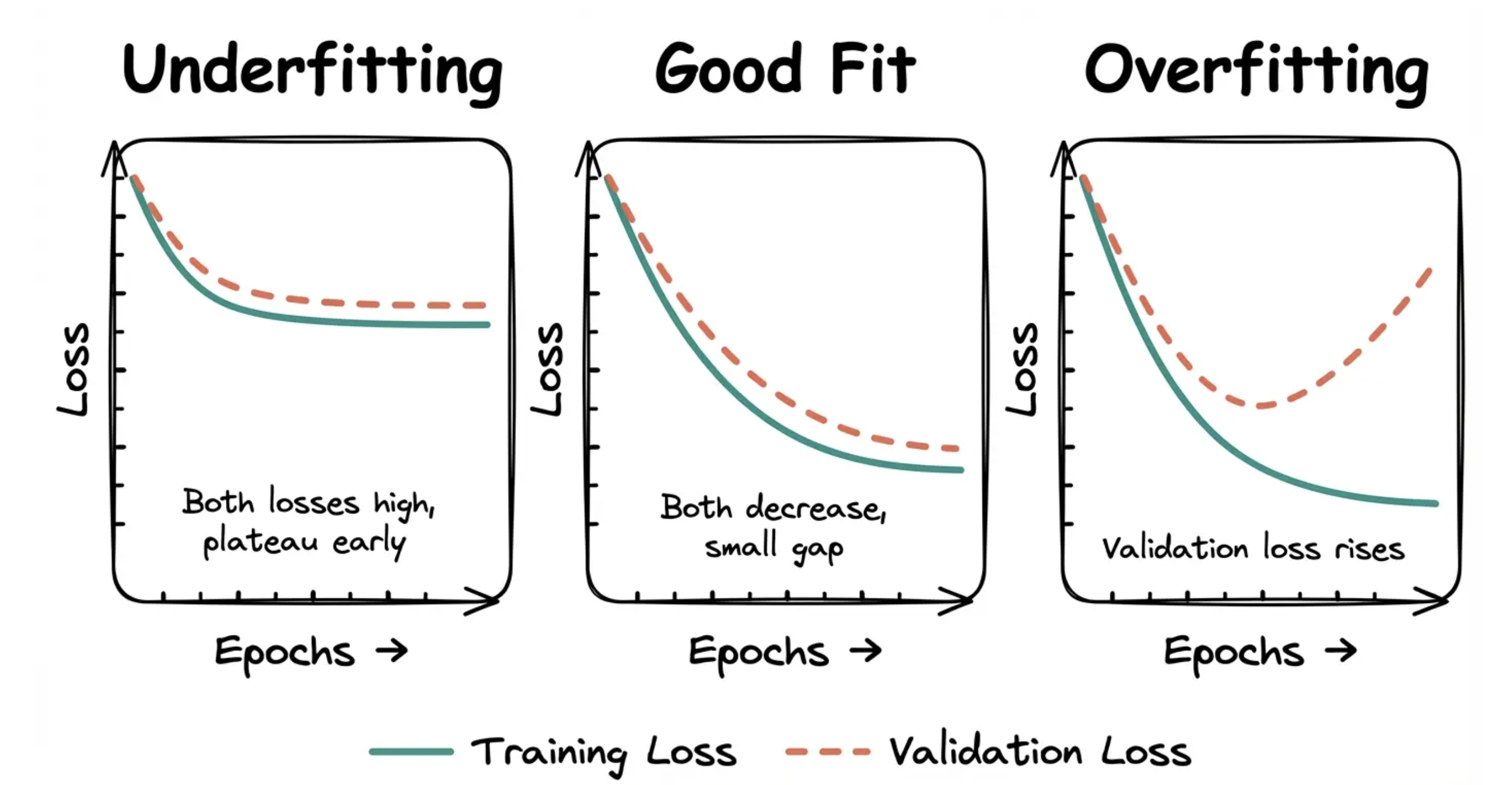
After training, we plot training loss and validation loss over epochs during training. Overfitting is easier to spot than underfitting if you're just looking at a single plot.

Underfitting: Both training and validation loss are high and decreasing slowly or plateauing early. The model isn't learning much.

Good fit: Training loss decreases steadily. Validation loss decreases and stays close to training loss. The gap between them is small.

Overfitting: Training loss keeps decreasing, but validation loss stops improving or starts increasing. The model is memorizing training data instead of generalizing.

Deciding which data to hold out for validation is an art. Holding out random data can work for some scenarios, but not others.

Consider an application where we're trying to predict stock returns. If we randomly hold out stock tickers, the model will still be able to "see" market-wide trends and crashes. Even if I didn't have Disney in my training set, if I knew the rest of the market dropped by 20% in April predicting the drop for Disney would be easy even if I didn't have April for Disney! But this gives me a false impression of my model's performance when I actually try to deploy it in the real world where I don't have access to the rest of the market.

In these instances, slicing by time is often a good approach. Train on all tickers from January through March, then validate on all tickers from April. Now the model has never seen April at all. If there is a market crash in April, it cannot cheat by learning that crash from other stocks in training. It has to generalize from past patterns only, which matches real deployment much better. But each problem may require slightly different treatment.

The other way to detect overfitting is your model does significantly worse in production than it did in your notebook or during training. In fact, a common question from interviewers is "let's assume you deploy this to production and it dramatically underperforms expectations, what do you do?"

Underfitting is usually a problem of picking the wrong model for the job. Interviewers are most often concerned with overfitting. But what can we do about it? Let's talk about some of the macro options before we get into the fine details of regularization.

How do you prevent overfitting?

• Manage model capacity and data requirements

• Transfer learning and small data

• Data augmentation, self and semi-supervised learning

What is model capacity and how do you manage it?

Model capacity is roughly how complex a function your model can represent, and typically practitioners will talk about it in terms of the number of trainable parameters in the model.

Two illustrative examples:

• A simple linear model has low capacity. It's very difficult for a linear model to learn a more complex function (even a sine wave) which means it's prone to underfitting. But on the plus side, it's almost impossible to overfit a reasonably-sized linear model.

• A deep neural network, on the other hand, has high capacity. It can learn a very complex function, but it's also prone to overfitting if you give it too little data.

Remember this: high-capacity models need more data to generalize well. If you give a huge model a tiny dataset, it will overfit almost immediately. It has so much freedom that it can memorize every training example instead of learning patterns.

A very common flag in ML design interviews are candidates who try to train huge models end-to-end with very limited data. This is usually an indication you haven't trained many models and interviewers are extremely sensitive to it.

Modern deep learning models have millions or billions of parameters. GPT-3 had 175 billion parameters. A typical image classifier might have 20-50 million. Each parameter is something the model can tune during training. More parameters mean more flexibility, which means more capacity to fit complex patterns. But it also means more capacity to fit noise. So one technique to mitigate overfitting is to use a smaller model.

What is transfer learning?

But what if we want the power of a large model with limited data? Training from scratch would overfit almost immediately. What do you do?

Transfer learning is one of the best approaches. The idea is simple: take a model that has already learned useful features from a large dataset and fine-tune it on your smaller dataset. A model pre-trained on millions of images has already learned to detect edges, textures, shapes, and objects. You don't need to relearn all that from scratch. Instead, you freeze most of the pre-trained weights and only train the final layers on your specific task.

This works across domains. BERT has 110 million parameters, but you can fine-tune it on just a few thousand examples for text classification because it's already learned language structure from billions of words. ResNet can classify your niche product images with a few hundred examples per category because it's already learned visual features from ImageNet.

In practice, the lower layers in neural networks learn general features (edges, common word patterns) while higher layers learn task-specific features (specific objects, sentiment). By transferring the general features, you only need to learn the task-specific parts from your limited data.

Most industrial systems will do a bit of surgery. They'll extract the parameters and layers from a pre-trained base model, freeze them during training (to avoid overfitting!), then add trainable layers on top for their specific tasks. This might be a new classification head, a LoRA (Low-Rank Adaptation) adapter, or an entirely different architecture.

What is data augmentation, self- and semi-supervised learning?

Two other techniques complement transfer learning when battling overfitting.

Data augmentation generates synthetic training examples by transforming your existing data (rotations, crops, paraphrasing) to expose the model to more variety. This is very common for computer vision models, but a bit trickier for NLP and other domains. Data augmentation works best when you have a good understanding of corruptions that can happen in your data.

While data augmentation can be very powerful in places, it's not a silver bullet. In many instances, generating diverse, high-signal synthetic examples can be harder than the original problem (e.g. of separating cats from dogs). Typically data augmentation is used to solve a particular problem (e.g. adding noise, rotations) rather than as a general solution to data scarcity.

If you're planning to use an LLM to generate data for your problem, a useful question to ask is "why not just use the LLM to generate the labels directly?" There are valid situations, but it's good to have the discussion to show you understand.

Self-supervised learning uses your large pool of unlabeled data to learn useful representations first, then fine-tunes on labeled examples. The model creates its own supervision signal from the data itself—predicting masked words, reconstructing corrupted images, or predicting the next frame in a video. Similar to transfer learning, but instead of starting from a pre-trained model, you start from scratch and use the unlabelled data to guide your training.

Semi-supervised learning takes a different approach: it uses a small amount of labeled data alongside a large pool of unlabeled data during training. Techniques like pseudo-labeling or consistency regularization let the model learn from both simultaneously. This works well when labeling is expensive but unlabeled data is plentiful.

In interviews, show you understand that small-data problems are common in production - new products, niche domains, and cold-start scenarios don't come with millions of labeled examples. Knowing when to reach for transfer learning versus when a simpler model is the right call is essential.

What is data drift and the types?

Data drift is when the distribution of your production data changes over time compared to your training data. Your model learned patterns from historical data, but the real world changed, and those patterns don't hold anymore.

This is different from overfitting. You might have a perfectly well-generalized model that performed great when you deployed it, but six months later it's failing because the data itself changed.

Types of Data Drift

Data drift can appear in different ways, but the story is the same: the training data is no longer a good representation of the production data.

Covariate shift happens when the distribution of your input features changes, but the relationship between features and labels stays the same. For example, a recommendation system trained on summer user behavior sees different patterns in winter. The features (time of day, categories browsed) have different distributions, but if you'd trained on winter data with the right labels, the model would still work.

Prior probability shift (or label drift) happens when the distribution of your target variable changes. Maybe you built a fraud detection model when fraud was 1% of transactions, but now it's 3%. The model's decision threshold might not be calibrated correctly anymore.

Concept drift is the nastiest type. The actual relationship between features and labels changes. User preferences evolve, competitor products launch, regulations change, or world events alter behavior. The patterns your model learned are just wrong now.

Depending on the problem, it's common for interviewers to ask about how to deal with this hairy issue. You'll want two pieces: detection and remediation.

How do you detect and handle feature drift?

Detecting Feature Drift

First, to detect data drift, there's a number of weapons in your arsenal. Mature production systems will use many of these:

Monitor prediction distributions: Track the distribution of your model's predictions over time. If your fraud model suddenly starts flagging 10x more transactions, something changed. Either fraud patterns shifted, or your input data distribution changed.

Monitor feature distributions: Track statistics on your input features. Calculate mean, variance, percentiles for numerical features. Track category frequencies for categorical features. Set up alerts when these drift beyond acceptable thresholds.

Monitor performance metrics: Track your model's actual performance on labeled production data. If accuracy, precision, or recall degrade over time, you've got drift. The challenge is getting ground truth labels quickly enough to catch drift before it does serious damage.

Model retraining cadence: If you're retraining regularly (weekly, monthly), compare performance on the same hold-out test set over time. Degrading performance on a fixed test set signals drift.

Data drift detection is hard and some teams try to aggressively remediate rather than detect it. Being able to talk about how you'd monitor is a useful way to show your understanding of the problem.

Handling Feature Drift

Once you've detected drift, what do you do?

The biggest thing is to retrain regularly. This, of course, is less common than you might assume in real teams partly because production pipelines are hard to get right. But retraining regularly ensures that your model has fresh, near-current data to learn from, minimizing the risk of drift. In an interview setting, it's free to suggest that you'll do the thing that people should be doing anyways, so start here.

Next, we need to consider approaches that carry tradeoffs.

Online learning is best for systems that need to very rapidly adapt to data drift. Some models, like logistic regression, can update continuously on new data as it arrives, but this is harder with deep learning. The risk is catastrophic forgetting: the model forgets old patterns while learning new ones. So you'll more typically see online learning when systems need to very quickly adapt to data drift. Fraud is a classic example of this.

A modern in-between approach is online embedding learning. In this approach we keep model weights frozen but have embeddings or parameters which are updated continuously. This is a prodigious engineering challenge, but required for the rapid adaptation that makes recommendation systems behind Tiktok and Instagram reels work (more on this in our Video Recommendations problem breakdown).

Less commonly used, but still valid are ensemble approaches. We keep multiple models trained on data from different time periods and weight their predictions based on which time period best matches current data. This hedges against drift but increases serving costs. Typically you'll have an ensemble for other reasons and some sort of multi-armed bandit or tournament to choose which model to use for new predictions.

Finally, for high-stakes applications, we can route uncertain predictions to humans for review with human-in-the-loop. Their feedback provides fresh training data that reflects current patterns.

If data drift is a concern for the problem you're solving, start with basic hygiene around retraining regularly and getting fresh labelled data. If there's still concerns, online learning approaches may be a good fit.

What is regularization?

We've talked about approaches to battle overfitting and data drift at the macro level, but what if we could force our models to learn more robust patterns in the first place? This is where regularization comes in.

Regularization improves generalization by constraining the model during training so it's more difficult to memorize noise. You're trading some training performance for better generalization on unseen data.

This helps both with overfitting during initial training and with building models that degrade more gracefully when drift happens. A well-regularized model that learned robust patterns tends to handle distribution shift better than one that memorized brittle correlations.

Dropout and Layer Normalization

Dropout randomly disables neurons during training. On each training step, every neuron has a probability p (like 0.5) of being turned off. This forces the network to learn redundant representations because it can't rely on any single neuron always being there.

At test time, all neurons are active but their outputs are scaled down by (1-p) to account for the fact that more neurons are firing than during training. Most frameworks use "inverted dropout" instead, which scales up surviving neurons by 1/(1-p) during training so no adjustment is needed at inference.

Layer normalization normalizes activations across features within each training example. It stabilizes training and has a mild regularization effect.

If you're proposing deep models, you're talking about dropout and layer normalization. Dropout is extremely effective for preventing overfitting in large networks.

You'll still see batch normalization (batchnorm) in older architectures and CNNs, but layer normalization has largely replaced it in transformers and modern architectures. Batchnorm normalizes across the batch dimension, which creates issues with small batch sizes and makes it awkward for sequence models where different positions shouldn't share statistics. Layer normalization avoids these problems by normalizing within each example independently.

L2 Regularization (Ridge / Weight Decay)

L2 regularization adds a penalty to the loss function proportional to the square of the weights. Large weights get penalized more than small ones.

This makes weights stay smaller and more evenly distributed. The model can't rely too heavily on any single feature, which prevents it from fitting noise.

When to use it: Almost always. L2 is the default regularization technique for most models. It's cheap, effective, and doesn't complicate training much.

In practice, you tune the regularization strength (often called lambda or alpha) on a validation set. Too much regularization and you underfit. Too little and you overfit.

In interviews, L2 regularization is the first regularization technique you should mention. It's simple, well-understood, and works across almost every model type.

L1 Regularization (Lasso)

Another approach is L1 regularization. This adds a penalty proportional to the absolute value of the weights. Unlike L2, L1 pushes weights all the way to zero, effectively performing feature selection.

The effect: sparse models where many weights are exactly zero. Only the most important features survive.

When to use it: When you have many features and suspect most aren't useful. L1 gives you interpretability by showing which features matter. It's common in linear models and logistic regression, less common in deep learning. L1 regularization can be really helpful in performance constrained scenarios: you can prune features (or sometimes weights) to get a simpler model that still performs well.

Early Stopping

Before, we noted that the graphs of overfit models tended to get better then start to perform worse as the model continues to train. We can exploit this. Early stopping is simple: stop training when validation performance stops improving. You monitor validation loss during training, and if it doesn't improve for N epochs, you halt and use the model from the best epoch.

This prevents the model from continuing to overfit after it's already learned the useful patterns.

When to use it: Always. Early stopping is free and effective. It's not a replacement for other regularization techniques, but it's a good safety net.

What are non-parametric approaches?

Non-parametric approaches are a class of statistical or machine learning methods that do not assume a specific form for the underlying data distribution. In other words, unlike parametric methods (like linear regression or Gaussian models), you don’t assume a fixed number of parameters or a predefined shape (like normal distribution) for the data.

This makes non-parametric methods flexible and useful when you don’t know the underlying distribution or the relationship is complex.

• No fixed number of parameters

  • Parametric models have a fixed structure (e.g., linear regression has coefficients for each feature)

  • Non-parametric models grow in complexity with the data (more data → more model capacity)

• Flexibility

  • Can fit very complex, non-linear patterns

  • Often more robust to unusual or unknown distributions

• Trade-offs

  • Usually need more data to perform well

  • Can be computationally expensive

  • Harder to interpret than simple parametric models

Type	Examples	Use Case
Density estimation	Kernel Density Estimation (KDE), Histogram	Estimate probability distribution without assuming a shape
Regression / Classification	k-Nearest Neighbors (k-NN), Decision Trees, Random Forests	Flexible prediction without assuming linearity
Hypothesis testing	Mann-Whitney U test, Wilcoxon signed-rank test	Compare groups without assuming normality
Clustering	DBSCAN, hierarchical clustering	Group data points without assuming cluster shapes
Ensemble methods	Random Forests, Gradient Boosted Trees	Non-linear decision boundaries for complex datasets

Think of parametric methods as trying to fit your data into a pre-made mold (e.g., line, Gaussian), whereas non-parametric methods let the data shape the model itself.

While non-parametric approaches can be a great optimization for many ML problems (and especially ones that have compute constraints), they're not without their drawbacks. The data we choose to index and include in our nearest neighbor search can have a big impact on the quality of our results. If we have a feedback loop in our system, we risk runaway feedback loops where we gradually index more and more benign data.

It's important that our system distinguishes ground truth labels provided by our investigators from labels generated by our system and weights these accordingly.

What are the categories of training data?

Ground Truth Labels

Our interviewer mentioned that investigators can manually verify accounts at a rate of hundreds per week. This represents our highest-quality data source, though it's extremely limited in scale. We should strategically use these labels for:

• Validating our model's performance on edge cases

• Creating test sets that reflect real-world bot sophistication

• Calibrating our confidence thresholds

Given the scarcity, we need to be strategic about which accounts we send for manual review focusing on those near decision boundaries (e.g. accounts that are close to the score threshold we choose to separate bots from non-bots) or representing new patterns.

User-Generated Signals

Beyond manual labels, the platform generates numerous signals that correlate with bot activity:

• Account Reports: When users flag accounts as suspicious, these provide noisy but scalable labels. We'd expect millions of reports compared to hundreds of manual reviews.

• Appeal Outcomes: When restricted accounts successfully appeal, this gives us high-confidence negative labels (accounts incorrectly flagged as bots).

• Spam/Abuse Reports: Content-level reports often correlate with the accounts producing that content being bots.

While these signals are noisier than manual reviews, their volume makes them invaluable for training larger models and detecting emerging patterns.

Network-Based Labels

We can leverage the social graph to propagate labels intelligently:

• IP Address Clustering: Accounts originating from known malicious IPs (from historical bot campaigns) provide additional positive labels

• Behavioral Similarity: Accounts exhibiting nearly identical activity patterns to confirmed bots likely represent coordinated campaigns

• Registration Patterns: Bulk account creation from similar sources often indicates bot farms

This approach helps us identify entire bot networks rather than individual accounts, though we must be careful not to propagate errors through the graph.

Synthetic Data Generation

Given the severe class imbalance (bots might represent <1% of accounts in the cleaned dataset), we can use generative approaches to augment our training data. Conditional GANs (like CALEB) can generate realistic bot behavior patterns across multiple dimensions:

• Temporal activity patterns

• Content generation styles

• Network formation behaviors

This helps our model learn to detect sophisticated bot patterns that might be underrepresented in our real data.

The adversarial nature of bot detection creates an interesting dynamic: as our detection improves, the bots we observe become more sophisticated (since simple ones are filtered out). This survival bias means our training data naturally shifts toward harder examples over time - both a blessing and a curse!

What are GANs?

A GAN (Generative Adversarial Network) is a type of deep learning model used for generating new, synthetic data that resembles a given dataset. It’s widely used in images, videos, audio, and other data types.

How it works (high-level)

A GAN consists of two neural networks that “compete” with each other:

1. Generator (G)

   • Tries to create fake data that looks like the real data.

   • Example: generate an image of a cat that looks realistic.

2. Discriminator (D)

   • Tries to distinguish real data from fake data.

   • Example: look at an image and say “real cat” vs “fake cat.”

Training process (adversarial learning):

• G produces fake data → D tries to classify real vs fake → feedback goes back to G → G improves → D improves → repeat

• Over time, the generator learns to produce data that’s hard for the discriminator to tell apart from real data.

Intuition

Think of it like a counterfeit money problem:

• Generator = counterfeiter

• Discriminator = police trying to detect fakes

• Both get better over time, and ideally, the counterfeiter becomes so good that the police can’t tell fake from real.

Applications

• Image generation: realistic faces (StyleGAN), artwork, deepfakes

• Data augmentation: generating synthetic datasets for training ML models

• Anomaly detection: train GAN on normal data; high reconstruction error signals anomalies

• Text/audio generation: music, speech, handwriting synthesis

Important notes for your context (invalid traffic detection / ML system design)

• GANs could theoretically be used to simulate synthetic traffic for testing anomaly detection systems.

• But they’re not typically core for this type of MLE role; focus more on classical ML, anomaly detection, and scalable pipelines.

What are the types of features to consider in bot detection?

Activity Patterns

Bots often exhibit activity patterns that differ from human users, even when trying to mimic natural behavior. Ideally these patterns are learned by our model, but in many cases expensive sequence models are not feasible to run on every action so hand-engineered features are a good compromise.

• Posting Cadence: Inter-event time distributions (time between posts, comments, likes)

• Click Timing Precision: Variance in reaction times to content

• Error Rates: Typos, corrections, and natural human mistakes

• Session Patterns: Duration and frequency of active sessions

• Circadian Rhythms: Activity distribution across hours/days (humans typically show clear daily patterns)

• Burst Detection: Sudden spikes in activity that exceed human capabilities

These features should be computed over multiple time windows (hourly, daily, weekly) to capture patterns at different scales. We'll use statistical measures like entropy and variance to quantify how "human-like" these patterns appear.

Content Signals

While sophisticated bots increasingly use AI-generated content (i.e. instead of posting the same content over and over), there remain detectable patterns:

• Semantic Diversity: Vocabulary richness and topic consistency across posts

• Duplication Signals: Exact or near-duplicate content (via embedding similarity)

• Language Quality Metrics: Grammar, coherence, and style consistency scores

We'll need to be careful here because not all repetitive or low-quality content comes from bots. These features work best in combination with others.

Instead of exclusively learning these features, we can keep track of bot-posted content and keep it indexed separately in an ANN vector store. Then, when content is posted, we can use the distance or count of nearby content to inform our model. This will help us avoid overfitting to content and reacts more quickly to new patterns than a model which needed to see content examples during training.

Content signals tend to be some of the weakest for bot detection because they're the easiest to fool/fake and often the most visible. If our systems are consistently taking down content that looks like X and not like Y, our adversaries will make more of Y and less of X!

This is less often the case for e.g. temporal activity patterns.

Network Topology Features

The social graph provides rich signals about account legitimacy. We might list a few for our interviewer.

• Follower/Following Ratios: Bots often have skewed ratios

• Network Growth Rate: Speed of connection formation

• Clustering Coefficients: How connected an account's connections are to each other

We can also compute graph embeddings that capture an account's position and role in the network structure.

Account Metadata

Basic account properties provide useful baseline signals:

• Registration Metadata: Account age, verification status, profile completeness

• Authentication Patterns: Login frequency, device diversity, location consistency

• Profile Elements: Username patterns, profile photo characteristics, bio quality

While bots are getting better at faking these, they remain useful especially for catching less sophisticated attacks.

Real-time Behavioral Signals

As our system operates, we can compute features based on how accounts interact with our detection:

• Detection History: How often this account has been flagged across different models

• Evasion Patterns: Changes in behavior after being flagged

• Appeal Behavior: Frequency and success rate of appeals

This creates a feedback loop where the bot's attempts to evade detection become signals themselves.

A critical consideration: many of these features won't be available immediately when an account is created. We need our model to handle missing data gracefully and potentially use different feature sets for new vs. established accounts. This temporal aspect of feature availability is something many candidates miss!

What are benchmark models?

A simple logistic regression fed with straightforward signals—post frequency, friend-request ratio, login geography, and so on is a good starting point. It trains in minutes, scores accounts in microseconds, and gives us a solid reality check. It's definitely not going to be the end of the road, but it shows we understand the need for a benchmark and can use it to layer on more sophistication where it matters.

A lightweight baseline isn’t throw-away work. It becomes the canary that warns when a future release quietly slips in the wrong direction.

How to choose model?

With a baseline in place, we pick tools that balance recall, precision, and speed. The biggest mistake candidates make here is assuming that one large content-focused multi-modal LLM is going to solve the problem. Bot detection is more of a challenge of assessing behavior than making determinations of content alone.

BAD:

Running a vision-and-language giant on every post is very expensive and misses some of the strongest features/signals we identified above like odd session rhythms, rapid IP swaps, bursts of follows, etc.

GOOD:

Combine two complementary views:

• Graph – who/what an account connects with and how densely.

• Sequence – what the account does over time.

This pairing spots lone-wolf spam accounts and coordinated botnets alike, all without parsing every bit of text or image content.

By utilizing a model that focuses on graph context (for coordinated operations) and action sequences, we can get a good sense of the behavior of the account.

How do you scale a bot detection model?

Our core, supervised bot detection model is computationally expensive, likely requiring GPUs to run efficiently. To reduce the compute footprint, we can implement several optimization strategies.

First, we can optimize the model. Quantization-aware training allows us to reduce memory requirements while maintaining accuracy. Since many bot accounts exhibit similar patterns, we can leverage caching for our encoders to avoid redundant computations. Account graph embeddings can be stored for a short period of time (potentially invalidated when major shifts happen) and activity pattern encodings can be cached and re-used.

In addition to core model optimization, we can also implement a two-stage architecture to reduce the number of accounts we need to run our expensive model on. This idea is common across most production systems and is a good way to handle scale. Rather than running our expensive graph-sequence model on every account, we implement a two-stage architecture:

1. Lightweight Filter: A fast logistic regression model using basic features (posting frequency, account age, device patterns) that quickly identifies obvious legitimate accounts

2. Heavy Model: Our full graph-sequence architecture reserved for accounts that pass the initial filter.

We'll train our lightweight filter in a teacher/student fashion to approximate the output of our more heavy model. This ensures alignment between the two models and serves our direct objective: finding those examples for which the heavy model will score high enough to trigger action.

This cascading approach reduces computational requirements by 80-90% while maintaining detection quality, and it gives us a tunable parameter to adjust resource consumption. If the system is under-resourced, we can dial up the threshold on the lightweight model to reduce the number of accounts we need to run the heavy model on (with some tradeoffs in effectiveness).