ALL Statistical Tests

ONE CATEGORICAL VARIABLE

What does the Pearson chi-square goodness-of-fit test evaluate?  (chisq.test() or goodnessOfFitTest())

It tests whether observed frequencies match a specified probability distribution.

• H₀: observed data are consistent with the specified distribution

• H₁: observed data are not consistent with the distribution

Typical use-case: are all levels of a categorical variable equally likely?

What are the null and alternative hypotheses?

• H₀: all class probabilities are equal

• H₁: not all class probabilities are equal

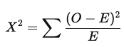
What is the chi-square test statistic, and how are degrees of freedom calculated?

O = observed frequency

E = expected frequency

• Larger X² values correspond to a lower probability of H₀ being true

• Degrees of freedom: k − 1

  • where k is the number of categories (levels of the categorical variable)

*exact rejection region depends on degrees of freedom

What is Cohen’s W, and how is it interpreted (3)? - Effect size

Cohen’s W measures the size of the deviation from the expected distribution:

• 0.10 = small effect

• 0.30 = medium effect

• 0.50 = large effect

*Larger values correspond to a larger deviation from the specified probability distribution under H0

What are the 2 assumptions of the chi-square goodness-of-fit test?

• Expected frequencies are all at least 5 in each category

  • in case of violation: use the exact goodness of fit test

• Observations are independent

TWO CATEGORICAL VARIABLES

What does the chi-square test of independence/association evaluate? (chisq.test() or associationTest())

It tests whether there is a relationship (association) between two categorical variables.

• H₀: the variables are independent (no association)

  • there is no relationship between the categorical variables

• H₁: the variables are not independent (association exists)

  • there is a relationship between the categorical variables

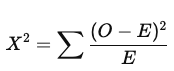
What is the test statistic for a chi-square test of independence and how are degrees of freedom calculated?

O = observed frequency

E = expected frequency

• Larger X² values correspond to lower probability of H₀ being true

Degrees of freedom: df = (r−1)(c−1)

• r = number of rows, c = number of columns in contingency table

  • the number of levels in both categorical variables

*exact rejection region depends on degrees of freedom

What is Cramer’s V and how is it interpreted? (cramersV())

• Cramer’s V measures the strength of association between two categorical variables

• Values range from 0 (no association) to 1 (perfect association).

Interpretation scale:

• 0–0.15: very weak

• 0.15–0.20: weak

• 0.20–0.25: moderate

• 0.25–0.30: moderately strong

• 0.30–0.35: strong

• 0.35–0.40: very strong

*larger values correspond to a larger deviation from the specified probability distribution under H0

What are the assumptions of the chi-square test of independence?

• Expected frequencies are all at least 5

  • if violated: use Fisher’s exact test (fisher.test())

• Observations are independent

  • if violated: use McNemar’s test (mcnemar.test())

ONE CONTINUOUS VARIABLE

What does a one-sample t-test evaluate? (t.test() or oneSampleTTest())

Formal name: Student’s t-test

It tests whether the mean of a sample differs significantly from a known or hypothesized population mean.

• H₀: population mean equals a specific value

• H₁: population mean does not equal a specific value

*If the population standard deviation is known: t-test becomes z-test

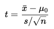
What is the t-test statistic, and how are degrees of freedom calculated?

• xˉ = sample mean

• μ0 = hypothesized population mean

• s = sample standard deviation

• n = sample size

Degrees of freedom: df = N − 1

• N is the number of observations in the dataset

*exact rejection regions depend on degrees of freedom

What is Cohen’s d and how is it interpreted?  (cohensD()) - Effect size

Cohen’s d measures the magnitude of difference between the sample mean and the population mean:

• 0.20 = small effect

• 0.50 = medium effect

• 0.80 = large effect

*larger values correspond to a greater difference from the value under H0

What are the 2 assumptions of a one-sample t-test?

• The continuous variable is normally distributed (check with Shapiro-Wilk test, histogram, Q-Q plot)

  • if normality is violated: use the Wilcoxon signed-rank test (wilcox.test())

• Observations are independent

What are key properties of the t-distribution used in t-tests?

• The t-distribution has thicker tails than the normal distribution (to account for extra uncertainty in small samples)

• As sample size increases, the t-distribution approaches the normal distribution

• Larger absolute t-values indicate more extreme results, corresponding to a lower probability of H₀ being true

TWO NON-PAIRED CONTINUOUS VARIABLES

What does an independent samples t-test evaluate? (t.test() or independentSamplesTTest())

Formal name: Student’s independent samples t-test

It compares the means of two independent groups to see if they are significantly different

• H₀: population means of both groups (samples) are equal

• H₁: population means of both groups (samples) are not equal

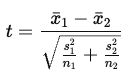
What is the test statistic for an independent samples t-test and how are degrees of freedom calculated?

Values further away from zero (i.e., higher absolute values) correspond to a lower probability of H0 being true

Degrees of freedom: df = N−2

• N is the total number of observations across both groups (in the data set)

*exact rejection regions depend on degrees of freedom

What is Cohen’s d and how is it interpreted for independent samples t-tests? (cohensD()) - Effect size

Cohen’s d measures the magnitude of difference between group means:

• 0.20 = small effect

• 0.50 = medium effect

• 0.80 = large effect

What are the 3 assumptions of the independent samples t-test?

• The continuous variable is normally distributed in both groups

  • Check with Shapiro-Wilk test, histogram, Q-Q plot

  • If violated: use Wilcoxon rank sum test (wilcox.test())

• Homoskedasticity: variances are equal between groups (the variance is the same in both groups)

  • Check with Levene’s test (leveneTest())

  • If violated: use Welch’s t-test

• Observations are independent

TWO PAIRED CONTINUOUS VARIABLES

What does a paired samples t-test evaluate? (t.test() or pairedSamplesTTest())

Formal name: Student’s paired samples t-test

It compares the means of two related groups (e.g., before vs. after measurements on the same subjects).

• H₀: the mean difference between the paired groups is zero

  • the difference between the population means for both samples is zero

• H₁: the mean difference is not zero

  • the difference between the population means for both samples is not zero

What is the test statistic for a paired samples t-test and how are degrees of freedom calculated?

• dˉ = mean of the differences

• sd​ = standard deviation of the differences

• n = number of paired observations

*Values further away from zero (i.e., higher absolute values) correspond to a lower probability of H0 being true

Degrees of freedom: df = N−1

• N is the number of observations in the data set

*exact rejection regions depend on degrees of freedom

What is Cohen’s d and how is it interpreted for paired samples t-tests? - Effect size

Cohen’s d measures the size of the mean difference:

• 0.20 = small effect

• 0.50 = medium effect

• 0.80 = large effect

*larger values correspond to a greater difference difference in means

What assumptions does the paired samples t-test have?

• The differences between paired observations are normally distributed

  • Check with: Shapiro-Wilk test, histogram, Q-Q plot

  • If normality is violated: use the Wilcoxon signed-rank test (wilcox.test())

(???? chat said:)

• Observations within pairs are related; observations across pairs are independent

CONTINUOUS VARIABLES FOR TWO OR MORE GROUPS

What does a one-way ANOVA test evaluate? (aov(), then summary())

Full name: analysis of variance

ANOVA tests whether three or more group means are significantly different.

• H₀: all population means are equal

  • the population means are the same for all groups

• H₁: at least one population mean is different

  • the population means are not the same for all groups

What is the ANOVA test statistic and how are degrees of freedom calculated?

Test statistic: F

• Higher F values = lower probability of H₀ being true

2 degrees of freedom:

• Between groups: G − 1

  • G = number of groups

• Within groups: N − G

  • N = total number of observations

*exact rejection regions depend on degrees of freedom

What do you do after a significant ANOVA?

Use post-hoc tests to determine which groups are significantly different from each other:

• Pairwise comparisons: TurkeyHSD() or posthocPairwiseT()

• Planned comparisons: for contrasts of a prior interest

  • Specify comparisons of interest

*Adjust p-values for multiple comparisons using Bonferroni correction: p′ = p*m  

• m = total number of comparisons

What is eta squared (η²) and how is it interpreted? - Effect size

Eta squared measures the proportion of variance explained by the group differences:

• 0.01: small

• 0.06: medium

• 0.14: large

*larger values correspond to more unequal means

• (Alternate scale: 0.02 / 0.13 / 0.26 from lecture slides) (?? sooo which scale)

What assumptions does ANOVA make?

• Normality of residuals: the residuals are normally distributed

  • Check with: Shapiro-Wilk test (shapiro.test()), histogram, QQ plot

  • If violated: use Kruskal-Wallis sum test (kruskal.test())

• Homogeneity of variance: the variance is the same in both groups

  • Check with: leveneTest())

  • If violated: use Welch’s one-way test (oneway.test())

• Independence of residuals: The residuals are independent

CONTINUOUS VARIABLES FOR MULTIPLE CATEGORICAL VARIABLES WITH TWO OR MORE GROUPS

What does a factorial ANOVA test? (aov(), then summary())

Full name: analysis of variance

A factorial ANOVA tests the effects of two or more categorical independent variables on a continuous dependent variable. It evaluates:

• Main effects of each factor

• Interaction effects between factors

What are the null and alternative hypotheses for a factorial ANOVA?

Multiple sets of null and alternative hypotheses:

• Main effect of predictor A:

  • H₀: all group means of A are equal

    • the population means are the same for all groups of predictor A

  • H₁: at least one group mean differs

    • the population means are not the same for all groups predictor A

• Main effect of predictor B:

  • H₀: all group means of B are equal

    • the population means are the same for all groups of predictor B

  • H₁: at least one group mean differs

    • the population means are not the same for all groups predictor B

• Interaction between predictor A and predictor B: (A*B????)

  • H₀: the effect of A is the same at all levels of B

    • the population means for predictor A are the same for all groups of predictor B

  • H₁: the effect of A differs depending on the level of B

    • the population means for predictor A are not the same for all groups predictor B

**Make sure you know what main effects and interaction effects look like in a graph (see Section 16.2 of the book)

What do you do after a significant main or interaction effect in ANOVA?

Use post-hoc tests to determine which groups are significantly different from each other:

• Pairwise comparisons (TukeyHSD() or posthocPairwiseT())

• Planned comparisons for contrasts of a prior interest:

*Adjust p-values for multiple comparisons using a Bonferroni correction: 𝑝′ = 𝑝*𝑚

• 𝑚 = the total number of comparisons

What is the test statistic and how are degrees of freedom calculated in factorial ANOVA?

Test statistic: F

• higher values correspond to a lower probability of H0 being true for a model term

Degrees of freedom:

• Factor A: R−1

  • R is the number of groups for predictor A

• Factor B: C−1

  • where C is the number of groups for predictor B

• Interaction A and B: (R−1)(C−1)

• Residuals: N − (R*C)

  • N is the total number of observations

*exact rejection regions depend on degrees of freedom

What is the relationship between sums of squares (SS), means of squares (MS), and the F-statistic in ANOVA?

• Sums of Squares (SS) measure the total variability:

  • SSbetween​: variability between group means

  • SSwithin (residual): variability within groups

• Mean Squares (MS) are averages of sums of squares: MS = SS / df​

• F-statistic is the ratio of these mean squares: F = MSbetween / MSwithin​​

A higher F-value suggests that between-group differences are large relative to within-group variation, which may indicate a significant effect.

What is partial eta squared, and how is it interpreted? (etaSquared()) - Effect size

Partial η² measures the proportion of variance explained by one factor or interaction while controlling for others (0-1): Apply to both main effects and interaction effects.

• 0.01 = small

• 0.06 = medium

• 0.14 = large

*larger values correspond to more unequal means

• Partial η² measures the effect size of individual model terms (main effects or interactions), controlling for other terms in the model

What are the assumptions of factorial ANOVA?

• Residuals are normally distributed

  • Check with: Shapiro-Wilk test (shapiro.test()), histogram, QQ plot

• Homogeneity of variance: The variance is the same in both groups

  • Check with: leveneTest()

• Residuals are independent