DCF Valuation Modelling

Compact DCF Model and Utility of DCFs

• Useful to construct compact DCFs as they:

  • help learn the main features of a DCF Model w/o the complexity

  • assist in decision making in situations where quick analysis is needed

• DCF Models are used to value businesses

• Business value depends on the quantity and timing of expected future cash flows

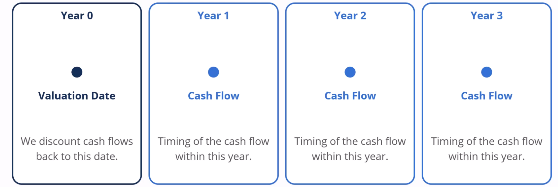
Important Dates

• Cash Flow Timing

  • dates within each year that case flows occur (middle, end)

  • simplified model typically uses EOY for simplicity however in a complete DCF cashflows can occur at ¼ of the year, ½ through the year, EOY

• Valuation Dates

  • Date that is set and used for valuation, all cash flow quantities will be adjusted for this date

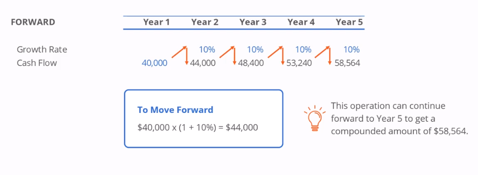
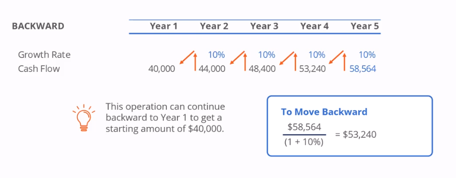
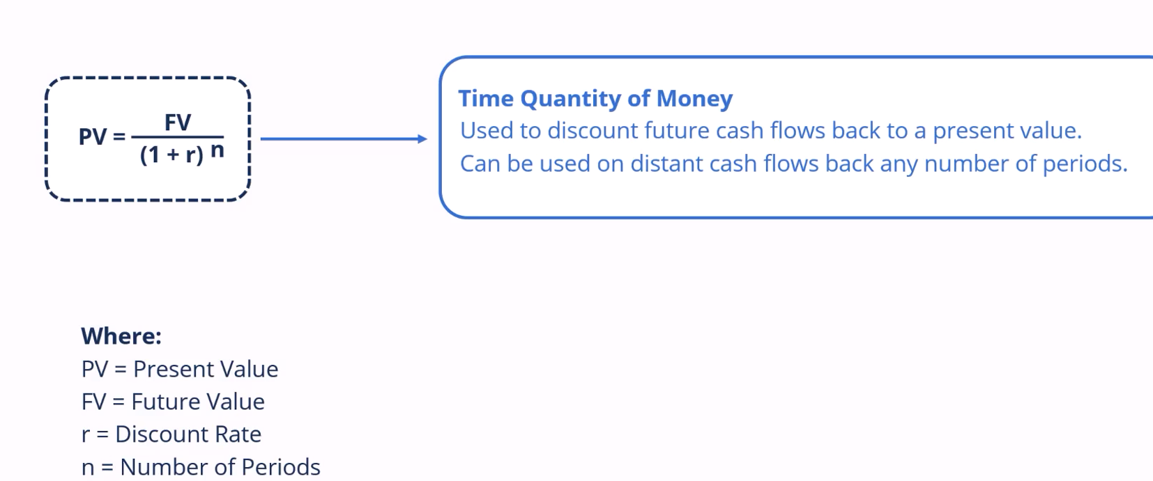
Time quantity of money

• Moving cash flows forward or backward is usually referred to as the time value of money

• for some reason CFI prefers time quantity of money as the quantity of money is changing over time

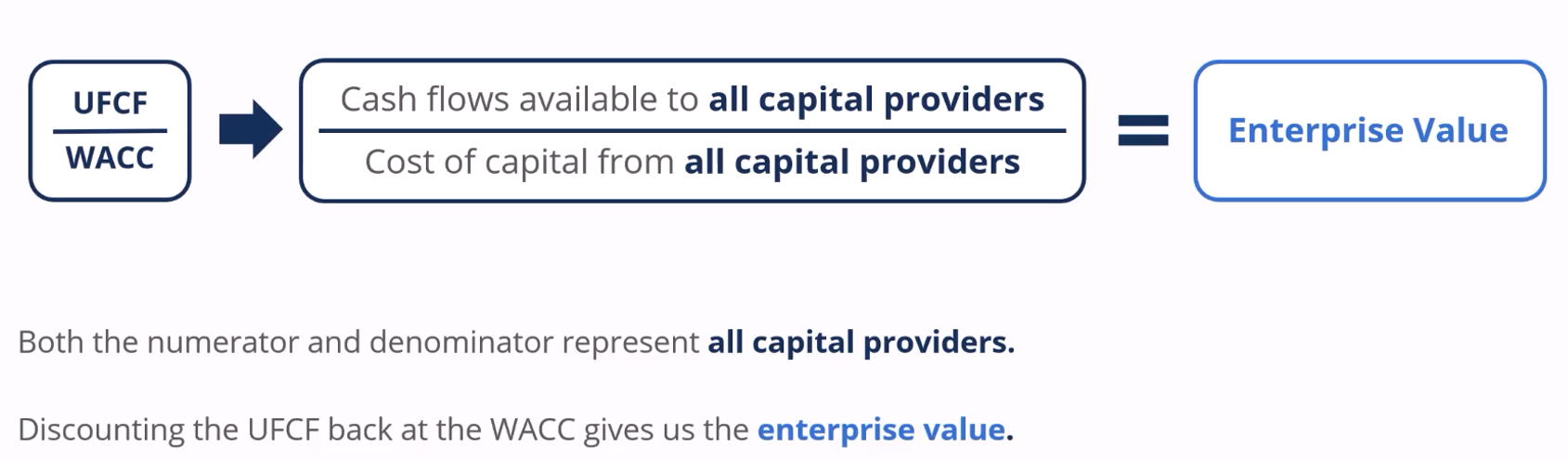
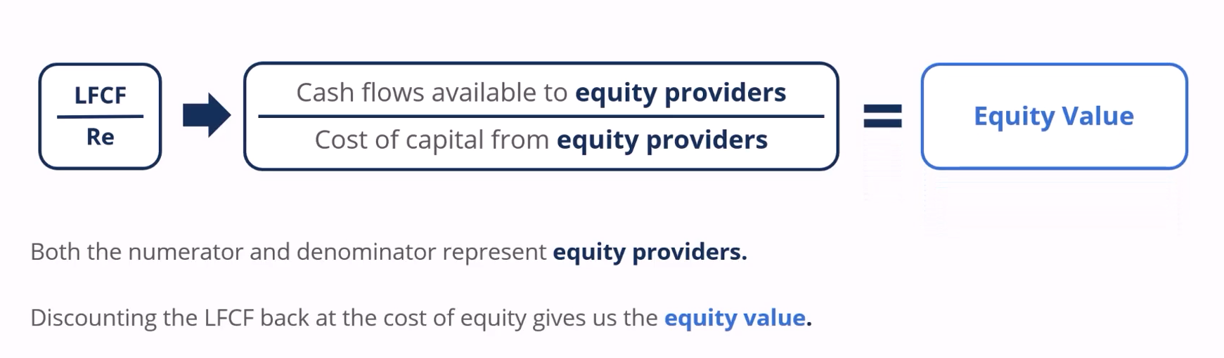
Choosing Cash Flows and Discount Rates

• Using the wrong cash flows and incorrect discount rates is a common mistake

• As a general rule:

• Consistency is needed between the numerator and denominator

• Both the numerator and denominator should represent all capital providers

• Discounting all UFCF back at the WACC gives the EV.

Forecasting Period

• Often assume that the business is a ongoing concern when doing a valuation analysis (aka operating continuously)

• This is done by separating cash flows into two parts

  • Discrete Forecasts

    • Shows the first few years when the company grows faster than the economy

    • Growth fore the company slows in later years as competitors enter the market

    • Eventually the company is mature and grows in line with the economy (point where TV occurs)

  • Terminal Value

    • covers the steady state period which continues indefinitely

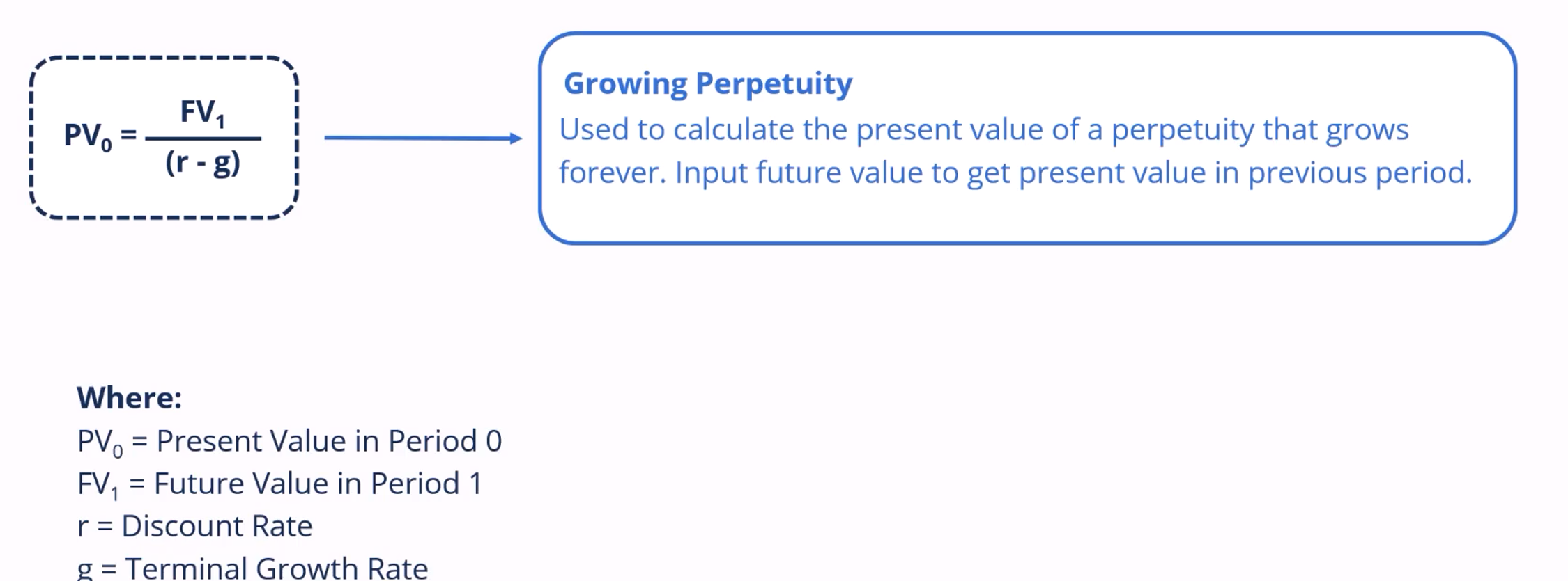
    • not practical to forecast the cash flows forever in the model, therefore a growing perpetuity formula is used to value the perpetual cash flows

Discrete Forecast

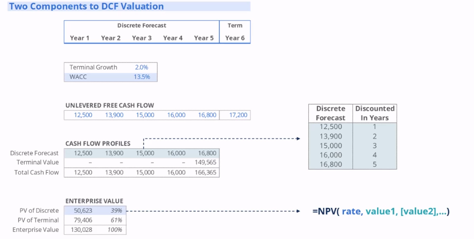
• Note that in this example the NPV function gives the present value at the end of year 0, however we don’t have any control over the timing of cash flows or the valuation date

• in this example, the function is taking the cash flows over the 5 year period and discounting it leading to a PV of over $50000

Terminal Value

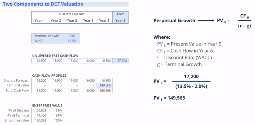
• assumes that the UFCF of 17200 is going to grow forever at a rate of 2% (Terminal Growth Rate)

• note that running the PV of a terminal UFCF will give a present value one year prior (aka last year of discrete forecast)

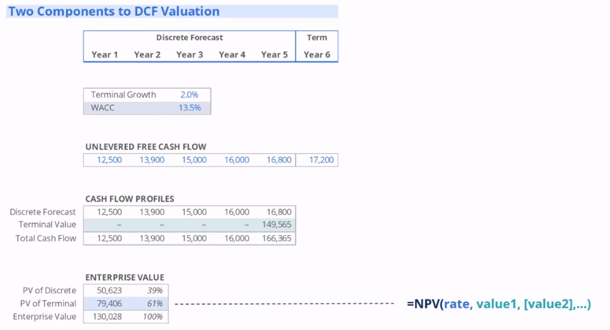
Enterprise Value

• Represents our view of the company’s value

• Calculated by:

  • PV of Discrete Forecast + PV of Terminal Value

Equity Value

• value that equity holders are entitled to

• Calculated by:

  • Enterprise Value - Net Debt

• Equity value for a singular shareholder can be calculated by:

  • Equity Value / Shares Outstanding

  • This represents our view of equity value per share and can be compared against the market price

Net Debt

• Net debt reflects cash being used to pay off debt

• Calculated by:

  • Total Debt - Cash

  • Enterprise Value – Equity Value (may not be a general rule)

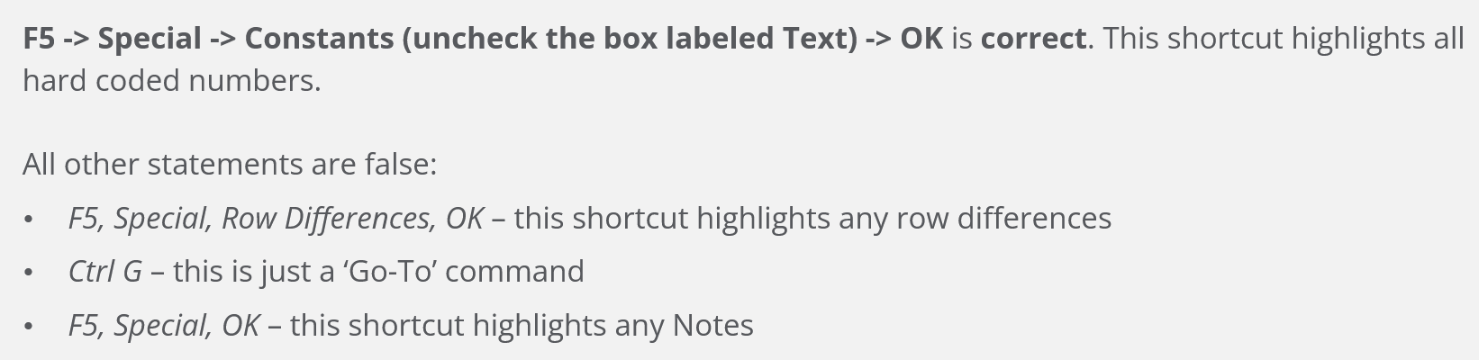
Cell Colours Shortcut

• Alt + H + H

• Can be used with multiple cells

• Remove cell colour: Alt + H + H + N (No Fill)

Group Tabs / Sheets Shortcut

• Careful with this shortcut as any actions taken in one tab / sheet will be replicated on all the sheets that are grouped

• Ctrl + Shift + Page Up / Page Down

Model Flow for DCF

• First is the UFCF Schedule which draws from EBITDA, Current Taxes, Capital Expenditure and Cash from Working Capital variables

  • Remember that Taxes, Capex and Cash from WC will be negative.

• UFCF will allow the calculation of the DCF schedule, split into the discrete forecast and terminal values

• Next is sensitivity analysis which allows for plotting enterprise value, varying it across different terminal growth rates and values for WACC, where we are then able to find equity value per share and the premium / discount

DCF Schedule

• After finding the UFCF, repeat the values for the discrete forecast

• The terminal value however uses the last cash flow divided by WACC - terminal growth rate

• After finding the discrete forecast and terminal value respectively, use the NPV functions to find the Enterprise Value

• Enterprise Value subtracting net debt can then be used to calculate Equity Value

• Equity Value per share can be calculated by dividing shares outstanding with Equity Value

• Equity Value per share can then be compared against current price to determine the premium/discount of the current share price relative to EVPS

Setting forecast dates

• Forecast dates can be odne using the Edate function in excel

• =Edate(Start Date, No of Months)

  • Start date is typically given by the first forecast date

Sensitivity Schedule Inputs

• Typically pull them from the DCF assumptions and includes:

  • terminal growth rate, WACC, Enterprise Value, Net Debt, Shares Outstanding, Current Price

• Typically placed on the very top of the schedule as they are meant to be informative for viewers

Sensitivity Table

• Start with the first table typically the EV table and drive the other tables using the first table

• Each table shows the Enterprise value, Equity Vlaue, EVPS, Premium/Discount to current price under different circumstances (WACC and terminal growth rate)

• Above the WACC and terminal growth rate we should also put the enterprise value in the top left corner (only for the first table)

• This is done by selecting the entire table (inc WACC and terminal growth rate): Alt + A + W + T

  • The row input cell must refer to the terminal growth rate

  • The column input cell must refer to the WACC in the DCF

  • Ensure that workbook calculation is set to automatic

  • Another Quick Check is the WACC and terminal growth rate we calculated being hard coded

• Typically, we also repeat the terminal growth rate and the WACC across all the sensitivity tables

Font Colour Keyboard Shortcut

• Select cell with data

• Alt + H + FC

Calculating Equity Value Table

• Essentially once we have derived all the enterprise value variables in the top table, it is possible to find all the equity value variables

• This is done by the same formula: Enterprise Value - Net Debt = Equity Value

• Ensure the Net Debt is locked using the F4 Function

Calculating Equity Value Per Share table

• Following the correct calculation of the equity value the equity value per share can be derived simply by:

  • Equity Value / Shares Outstanding

  • Ensure that shares outstanding variable is locked

Calculating premium/discount to current price table

• Following the calculation of the equity value per share the premium / discount can simply be derived by

  • Equity Value Per Share / Current Price - 1

  • Ensure that current price variable is locked

Data Table Important takeaways

• Ensure that calculation options are always running on automatic by default

• if there are a number of data tables running inside one model, it may be necessary to select the calculation option running on automatic except for data tables

  • This will mean that the F9 key will need to be refreshed to update

• The Y and X axis cannot move under any circumstances

  • This can be somewhat mitigated by hardcoding the WACC and Terminal Growth Value manually to centre the table

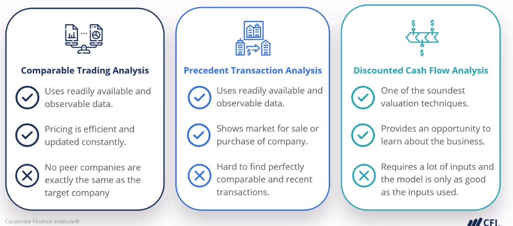
Valuation Techniques

• Three most common analysis techniques

  • Comparable Trading Analysis

    • looks at the valuation for similar peer companies that are publicly traded

    • relative valuation technique, as the target company is valued relative to where its peers are trading in public markets

  • Precedent Transaction Analysis

    • looks at the acquisition prices for similar peer companies in recent transactions

    • relative valuation technique as the target company is valued to where its peers have been acquired in past transactions

  • DCF Analysis

    • builds a model of the company to get the present value of all the company’s future free cash flows

    • absolute valuation technique, aka the intrinsic valuation technique, the value of peers is not considered in this process

Various Views of Value

• Comparable Trading Analysis

  • Market participants move the stock prices for peer companies so this technique shows their view

• Precedent Transaction Analysis

  • Previous buyers set acquisition prices, so this technique shows their collective view

• DCF Analysis

  • One builds the DCF model, select the inputs, therefore outputting “your view”

Advantages and Disadvantages of the techniques

Importance of model design

Upfront model design is critically important as:

• will result in a better financial model in the end

• will save large amounts of time on the model build

Why model businesses

• Modelling provides a deeper understanding of a business as modelling essentially forces you to understand all aspects of the business

• Start by understanding how it generates revenue or its cost structure in terms of variable and fixed costs, furthermore we also need to understand tax regulations and the company’s obligations (current or deferred)

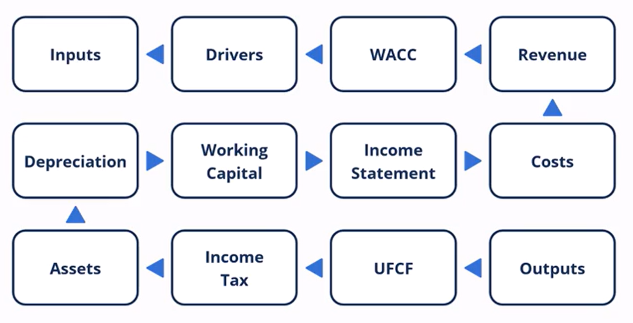
Model Design

• Start by thinking about inputs needed for the model

• Once gathered think about the calculations needed to lead us to the outputs

• In a linear flow we are going from the inputs, calculations all the way to the outputs

The role of financial models

• Decision Making

  • Financial decisions can be very complex, therefore models are important tools to assist with decision making

• Communication

  • Financial models must be easy for other to understand, dashboards are necessary so that figures can be clearly and easily communicated

Preferred Model Design

Using a DCF as the prime example, we are trying to make an informed decision about the valuation of a company

• The preferred method is to design using the opposite order, designing backward ensures all schedules support the outputs

• This also ensures the right level of detail through the financial model

Preferred model layout (communications perspective)

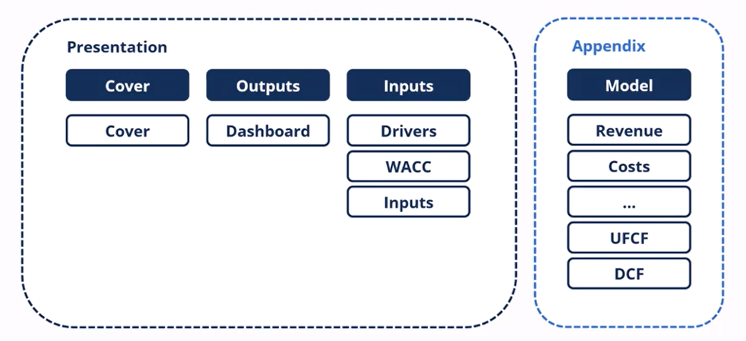
• Cover:

  • Typically consists of the business name, date, legal disclaimers and possibly model alerts

  • Sets the stage for the model and lets the readers know that the model has been formatted to be an effective financial presentation

• Dashboard

  • shows all the outputs and summarises the results from the inputs

• Inputs

  • consists of the drivers, WACC and inputs that are the engine of the model

• Appendix

  • large number of schedules that are driving all the calculations and formulas inside the model

  • this is gonna show everything in detail and how we’ve come to a decision

Building Blocks and how to employ them

• Should always think of models in a modular fashion made up of building blocks

• This reduces the difficulty and also enhances learning potential as one can simply practice one particular building block to get really proficient

How to save building blocks

• Those engaged in modelling typically have portfolios of schedules that facilitate model construction

• These are often referred to as building blocks, they might include schedules for claculating revenue, costs or taxes

• this allows to approach financial modelling in a modular fashion made up of a collection of schedules

• Once the schedule has been built and properly reviewed for integrity, they can be saved in a single excel file or multiple excel file with singular schedules for easy usage.

Understanding Drivers

• Model drivers are the most important inputs in the financial model, therefore we need to test how the model reacts when the drivers move

• evaluating the importance of the model inputs

  • isolate the drivers so that we can test how the model reacts to them

  • need to separate model drivers from other less important inputs

  • model drivers are volatile and have a significant impact on model outputs

  • identifying the drivers requires detailed knowledge of the business

Testing model drivers

• using an example, sales volume and sales price can be volatile and may have large impacts on the business

• therefore the first step is identifying the model drivers through conversations with the business owners and understanding the business

• the next logical step is to consider a minimum and maximum value for the drivers (best and worst case)

• this can be used to find and estimate a base case

• only the model drivers need to be tested with switches this way as errors can create large deviations

Choose Function

• Used to switch between wors, base and best case scenarios for an input driver (sales volume growth for example)

• Formula:

• =Choose(Index Number/Switch, Value 1, Value 2, Value 3)

  • Values are the best, base and worst case

Index Function

• Formula:

• =Index(Array,Row_Num)

  • Array will be the cases

  • Row numbers will be the driver switch cell

Combo Box

• Developer tab needed, which can be done through excel options

  • Alt + F + T

  • Customise ribbon → Developer tab check

• Once developer tab is available as an option, select the insert function and combo box

• Once a combo box has been created, select format

  • Input range should be the best, base and worst case variables

  • Cell link should be the driver switch cell

  • Errors will occur as the program will put a 0 by default

Macabacus library function

• Bring up library manager for macabacus → create a personal or corporate shared library → group schedules according to type (operational, financial)

• this would allow an easy way to access lots of schedules quickly across the whole organisation

Macabacus Uploading to library

• Select the entire schedule → Macabacus ribbon → settings → library manager → tables → new groups / within a group → publish

Macabacus inserting tables into sheets

• Typically start by clicking library → tables → library should pop up with library of schedules → simply double click to insert the model into the sheet

Isolating the schedule for uploads

• can be done using the flatten option on macabacus

• the function will replace all worksheets referencing other workbooks or worksheets with values

Macabacus show all precedents

• Ctrl + Alt + [ to initiate

• Ctrl = Alt + \ to clear

Macabacus format colour

• Using format and colour under the macabacus tab, select format → colour → font colours → autocolour sheet

• this will automatically make all formulas black and all inputs blue

Operational Schedules

• used to model the operational movements of a business

• typically positioned on the top of the model tab in a DCF worksheet

Current Taxes

• “current” is an accounting term meaning in the current period, also often thought of as cash taxes

• these are the amounts that are paid to the government as tax payments

• these represent the physical cash outflows from the company

• important for DCF as they can be used to calculate UFCF values

Deferred taxes

• Are essentially “non-cash” taxes, amount that the company will have to pay at some point in the future

• Most jurisdictions will offer these deferred taxes in the form of accelerated depreciation (done by adding accounting depreciation and subtracting tax depreciation to lead to a lower payable balance)

• Some jurisdictions also offer companies the ability to carry a tax loss forward into the future (credits that can be used to minimise the tax company pays)

Total Taxes

• Simply the current taxes + deferred taxes

• Income statements often only show one line for the total taxes, however it is important to note that many companies will have current and deferred taxes

• this can be identified in the cash flow statement particularly cash from operations where deferred taxes will be added back to net income

Levered Tax Schedule

• Starts with EBT

• Shows taxes that are payable when the company has debt in it’s capital structure

• Needed to calculate tax lines in the income statements

Unlevered Tax Schedule

• Starts with EBIT

• Shows taxes that are payable excluding debt in the company’s capital structure

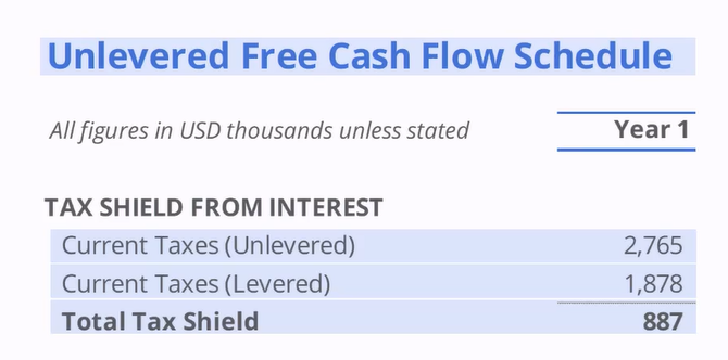
• Needed to calculate the tax shield

Tax Shield Calculation

• the tax shield is essentially the tax savings for the company when it uses debt to finance part of it’s operations resulting in an overall lower taxable income for the company hence the “shield”

EBITDA Method for calculating UFCF

• more common in capital market groups

• shorter and uses EBITDA which is a common measure of profitability

• method is also shorter as it starts with an unlevered term and ends with an unlevered term

Net Income Method for calculating UFCF

• method is longer as it starts with a levered term and ends with an unlevered term

• the unlevering is done by adding the interest and subtracting the tax shield

  • the tax shield being the difference between the amount of cash taxes saved by having debt in the capital structure

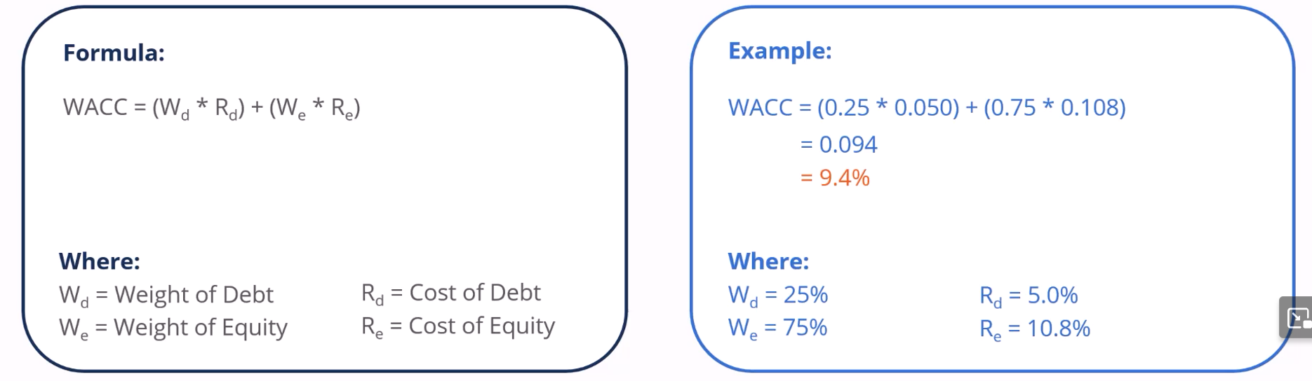
WACC Formula

• Discount rate that is used to discount the UFCF

• WACC must represent the cost of capital from all capital providers (debt and equity)

• Typically debt has a lower weight than equity

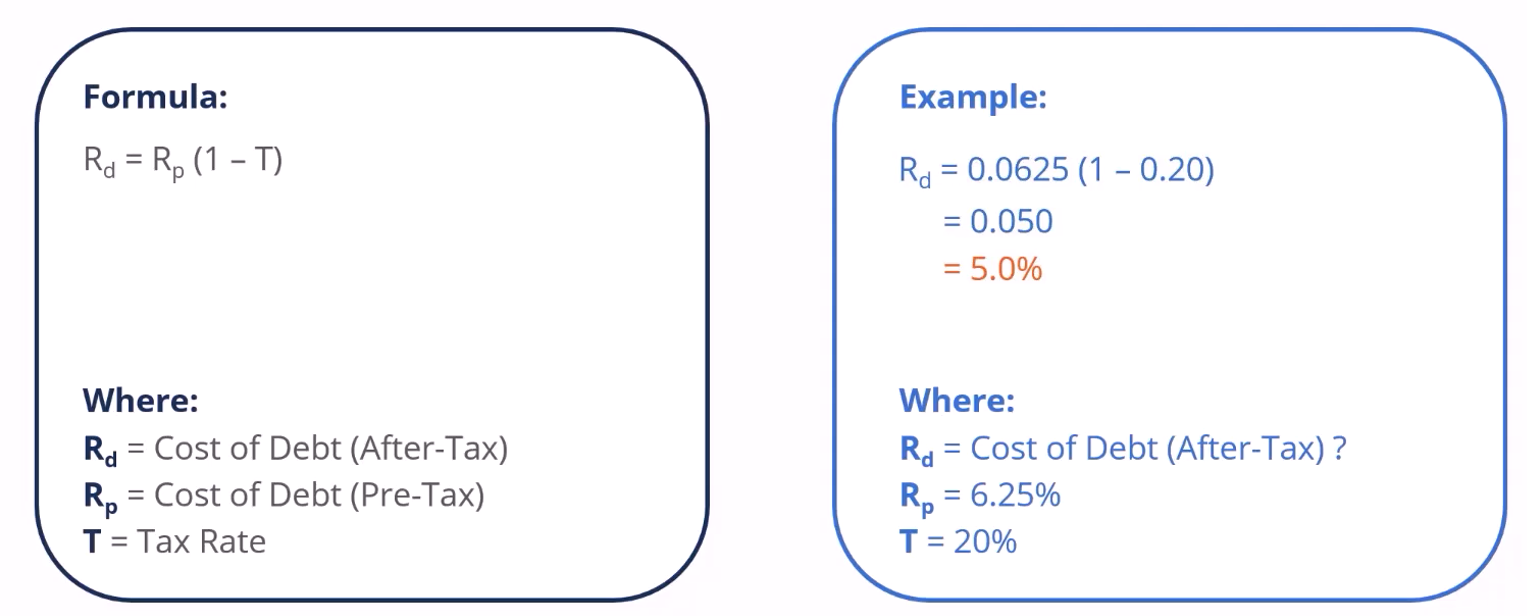
Cost of Debt Formula

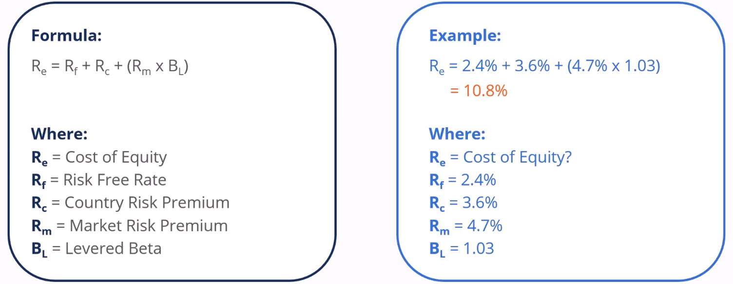
Cost of Equity Formula

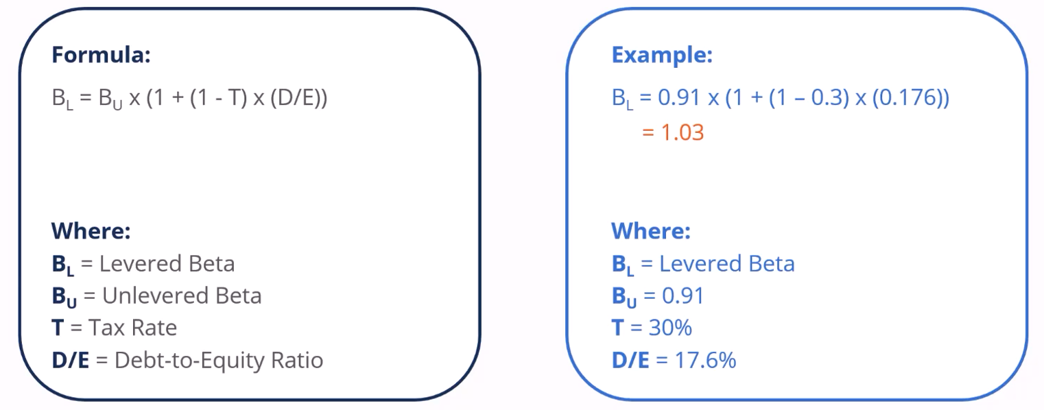
Levered Beta Formula

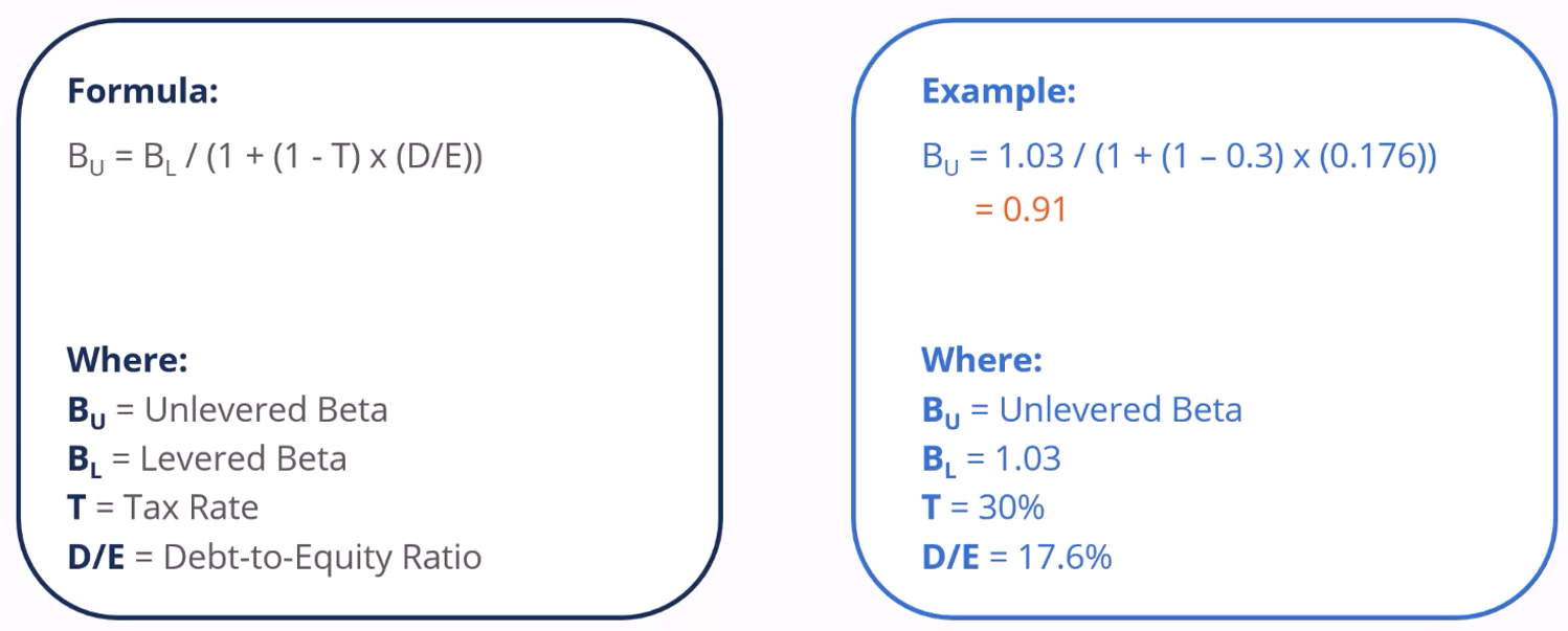
Unlevered Beta Formula

Equity Risk Premium

• Can be calculated by Levered Beta * Market Risk Premium

After Tax Cost of Debt

• Can be calculated by Pre Tax Cost of Debt * (1 - Tax Rate)

Model Alert for WACC and terminal growth

• Essentially used for ensuring that the terminal growth rate is not equal or supercedes the WACC, as otherwise the equation (GGM) would not work

• Can be constructed by an if function:

  • IF(Terminal Growth Rate > WACC), 1, 0

• Can be further improved with custom format cells (Ctrl +1)

  • [=0],"No"_);[=1],"Yes"

• Can also be improved with conditional formatting (Alt + H + L + N)

  • Select the cell and condition this case being “1”

  • Format by Colour

  • Select Colour

Components to forecasting well for DCFs

• It is critical that DCFs are able to forecast forever, this is done in 2 components

  • Discrete Forecast

    • This forecast is till the steady state where the company’s growth will outpace the economy’s growth

  • Terminal Forecast

    • This forecast is theoretically till forever and is where the company’s growth will be identical to the growth rate of the economy as the business matures

    • Important to be accurate with the terminal value as it repeats and grows forever and will carry a heavy weight in the valuation of the company

Key Timings for DCFs

• Understanding and determining the timing of cash flow and the valuation date

• Valuation dates can be set at any period within the first period (typically at the end or the beginning of the period when doing valuation work)

• However for cash flows, it may be useful to understand the underlying business, a business that generates most of its revenue in Q4 will have timings at the center of the 4th Quarter

• Businesses with no seasonality meanwhile would generate its cash flows evenly resulting in a timing in the middle of the year shown below

Dates to consider

• Fiscal Year End

  • date of the fiscal year end for the company

  • date can be easily found in the financial statements

  • common to see the same month and day every year

• Cash Flow Timing

  • date in which the cash flow is expected to occur

  • this could be closer to the fiscal year end if Q4 is seasonally strong

  • Between two fiscal year dates if there is no seasonality

• Valuation Date

  • Date in which all cash flows are discounted into

  • Date is set by the model building team

  • Present Value of the business will be as of this date

Present Value / time quantity of money formula

Growing Perpetuity Formula

Edate Function

• Useful for filling out discrete forecast and terminal forecast tables with fiscal year end and cash flow timing data

• Formula

  • =EDATE(Starting Date Cell, Months usually 12)

Unadjusted Cash Flow

• The discrete forecast is simply the UFCF copied and pasted

• The terminal value can be found by using the growth perpetuity method

  • Terminal UFCF / (WACC - Terminal Growth)

Partial Period Adjustment

• Companies may oftentimes have a fiscal year end date that is different hence the need to do partial adjustments

• This is because from the valuation date we are only looking into the future hence we are ignoring the data prior to the valuation date

• Can be calculated using the YEARFRAC formula

  • YEARFRAC(Fiscal Year End, Valuation Date)

Discounting using YEARFRAC

• YEARFRAC can also be used with discounting

• This is done by inputting the formula

  • Previous Cell + YearFrac(Cash Flow Timing, Valuation Date)

• Using the TQM formula we are then able to find the discrete forecast and terminal value

XNPV Function

• Formula is as follows:

  • XNPV(WACC, Undiscounted Cash Flows including valuation date and all dates including valuation dates)

• it is important to have the first cash flow as 0, it will correspond to the valuation date

• The manual and XNPV calculations of Enterprise Value may differ due to the treatment of leap years by the function and the manual method

Finding Percentages of Discrete and Terminal

• This may be necessary to calculate and it is done by simply adding the discounted discrete forecasts for the PV of discrete

• PV of terminal is calculated by taking the discounted terminal value

• EV is obviously the sum of both these values and we can then find the contributions of both the TV and Discrete

• Terminal tends to be higher as it stretches to infinity

Terminal Value using multiple method

• Multiply EBITDA of the final term with the multiple for the terminal value

• However there might be some cases where FYE doesnt align with the final cash flow timing, in this case we might have to find terminal adjustment

• This terminal adjustment is calculated by the yearfrac function between FYE and the final cash flow timing

• Afterwards the terminal value would be adjusted with the formula:

  • (EBITDA x Multiple) / (1+WACC)^Terminal Adjustment

  • This in turn will discount the terminal value by the correct amount of time

Model Dashboards

• Model drivers are critical inputs that must be shown

• A toggle is often provided to change these drivers as well

• A DCF dashboard would need to have a toggle to show the range of enterprise and equity values

• A range of valuations are normal as different views and valuations may differ for the WACC and growth rate of the company

  • These can be done using data tables

Data Tables to find Enterprise Value

• First the top left will typically have an area to input the enterprise value into the table

  • It is important to ensure that the enterprise value matches the method used such as perpetuity/multiple

• After this select the entire table and create a data table using the shortcut

  • Alt + A + W + T / Alt + D + T

  • Row Input Cell: Terminal Growth Rate (select the cell with the TGR),

  • Column Input Cell: WACC (select the cell with WACC)

  • Ensure workbook calculation is set to automatic

Master Switch Linking between outputs and inputs

• Typically done by going to input side switch and linking it to the output side switch

• Change the input side combo box to the output side cell

• Create a combo box for the output side and select the range as usual being the best, base and worst case while the cell link would be set for the switch

1 Dimensional Data Tables

• This is used to calculate the best, base and worst case for enterprise value

• Select EV and the numbers 1,2,3 signifying the cases

• Column being the EV

• Row input cell being the numbers

• This would allow easily calculation for equity value and equity value per share

Checks and Balances