Relational Algebra for IDM

Concepts of RA but with a focus on databases for the IDM course

What is Arity in DBMS?

In DBMS, arity refers to the number of attributes (aka columns) in a relation (a table).

For example, if a table Employee has columns: EmployeeID, Name, Age, and Department, then the arity of this relation is 4.

What is Cardinality in DBMS?

In DBMS, Cardinality is the number of tuples (rows) in a relation (table). It reflects the dataset size.

Example:

EmployeeID	Name	Age	Department
101	Alice	30	HR
102	Bob	25	IT
103	Charlie	28	Finance

Here the cardinality is 3 & the arity is 4.

Projection

• Purpose: To select specific columns (attributes) from a relation

• Notation:

  πattribute1,attribute2,…(R)

  where R is a relation and the attributes listed are those to keep. (It will remove duplicates since relations are sets)

Example:

From the Employee relation, to get just the Name and Department of all employees:

π Name, Department(Employee)

Result: A relation with only two columns, Name and Department.

Selection

• Purpose: To filter rows (tuples) from a relation based on a specified condition.

• Notation:

  σcondition(R)

  where R is a relation and condition is a logical expression on attributes.

Example:

Example:
Given a relation Employee with attributes (EmployeeID, Name, Age, Department):

To select employees from the IT department:

σ Department=′IT′(Employee)

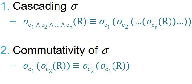
Result: Only rows where Department is 'IT' are included.

Algebraic properties of Selections σ

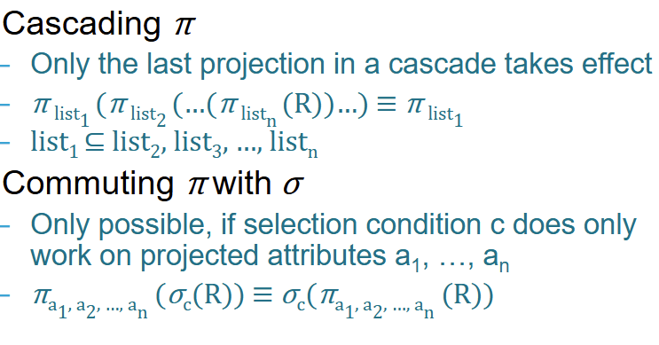
Algebraic properties of Projections π

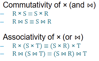
Algebraic properties of Joins & Cartesian products

—> Side note: This only works if the JOIN happens on tables with joint attributes

What happens if you try to do a NATURAL JOIN between 2 tables without shared attributes

It actually becomes a Cartesian Product!!

How can you rewrite an inner join as a Cartesian Product?

R ⋈c1 S

By combining it with a select:

σc1(R × S)

The same can be applied with other join operations

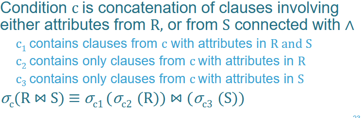
Give an example & explain the rewriting for “Pushing Selections Down in JOINS”

—> Do the selections and Projections as early as possible

For example:
Imagine we have two tables:

1. Students ($R$): ID, Name, Major

2. Enrollment ($S$): StudentID, Course, Grade

We want to find students who are Computer Science majors and have a Grade of 'A' in a course, where the ID matches the StudentID.

Our total condition c is: (Major = 'CS' AND Grade = 'A' AND ID = StudentID)

Normally we’d do:

\sigma_{(Major='CS' \wedge Grade='A' \wedge ID=StudentID)} (Students \bowtie Enrollment)

But now we can rewrite to:
\sigma_{(ID=StudentID)} (\sigma_{(Major='CS')}(Students) \bowtie \sigma_{(Grade='A')}(Enrollment))

This is more efficient because we’re selecting less data to start with

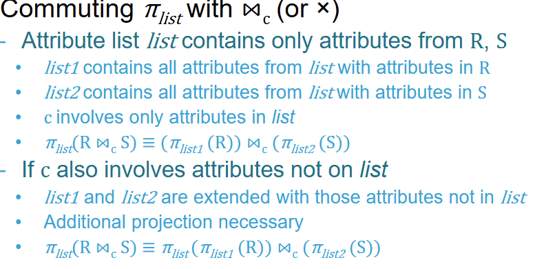
Give an example & explain the rewriting for “Pushing Projections Down in JOINS”

Same logic as with Selections —> only thing to add is that you can’t project everything! The attributes that are responsible for the JOIN condition can only be projected AFTER the JOIN.

Example:
We have two tables in a company database:

• Departments ($D$): {DeptID, DeptName, Location, Budget}

• Projects ($P$): {ProjectID, ProjectName, DeptID, Deadline}

The Goal: We want a list showing the DeptName and the ProjectName for all projects.

Normal, unoptimized way:
\pi_{DeptName,ProjectName}(Departments\bowtie_{D.DeptID=P.DeptID}Projects)

But now we optimize:
\pi_{DeptName,ProjectName}(\pi_{DeptName,DeptID}(Departments)\bowtie(\pi_{ProjectName,DeptID}(Projects)))

Note that we still DeptID within our JOIN so we still project it but get rid of it in our final projection!

What is pipelining of Unary Operators?

Pipelining is a method where the output of one relational algebra operation is passed directly to the next operation as a stream of data, without ever saving the intermediate results to a temporary file on the disk (which is called "materialization").

When we talk about unary operators (operators that take only one table as input, like Selection and Projection ), pipelining is extremely efficient.

Let's look at a query for our Students table:

\pi_{Name}(\sigma_{Major='CS'}(Students))

• Without Pipelining (Materialization): 1. The system scans the whole table and finds all CS majors.

  2. It writes those rows to a temporary table on the disk.

  3. It then reads that temporary table back into memory.

  4. It removes all columns except Name and shows you the result.

• With Pipelining:

  1. The system reads one row.

  2. Is it a CS major? Yes.

  3. It immediately "strips" the other columns and keeps just the Name.

  4. It moves to the next row.

Why is this better?

Pipelining saves a massive amount of I/O (Input/Output) because it avoids writing to and reading from the hard drive for every step.

Explain the 2 ways pipelining can happen

Demand Driven (aka Pull):

• Top-down approach

• Mechanism: The operation at the top of the query tree "demands" a tuple from the operation below it.

• Buffer: Each operation uses its buffer to store just enough tuples to satisfy the request from above.

• Key Benefit: It is very efficient with memory because we only process exactly what the final output needs at that moment.

Producer Driven (aka Push):

• Bottom-up approach

• Mechanism: The lower operations (producers) process tuples as fast as they can and "push" them into the input buffer of the operation above them.

• Buffer: The buffers here are filled eagerly. If the operator above is slow, the producer keeps filling the buffer until it’s full.

• Key Benefit: It can be faster on multi-core systems because every "station" on the assembly line works at its maximum speed whenever data is available.

Give the restrictions of pipelining:

Since pipelining restricts the available operations it only works well for certain cases:

Works well for:

• Selection, projection (aka unary operators)

• Index nested loop joins

Does not work well:

• Sorting, aggregated functions

• Merge joins

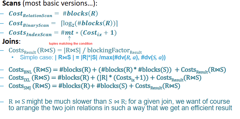
What is a Relation Scan?

Used to locate and retrieve records that fulfil a selection condition

A basic linear search over the entire relation. Its cost is simply the total number of blocks in the relation: #blocksR

What is Binary Scan / Search?

A more efficient search (typically on sorted data) with a logarithmic cost: log2​(#blocksR)

• Only applicable if the selection is an equality on the ordered attribute

• This is typically the case if the selection attribute is a primary key

What is Index Scan?

Uses an existing database index to find records. Its cost is calculated asCostForIndex + CostsForRetrievingResults

—> The cost of the results are often:

• for B-trees: the Height of the tree

• for hash indexes: a constant + number of page that overflow the list

What’s the best scan option for conditional selection?

Depending on what you have available:

Primary Index (Sorted on the attribute) exists:

• For "Greater Than" or "Greater Than or Equal To" (> or ≥): The system uses the index to find the very first matching value, and then simply scans the rest of the relation from that point forward.

• For "Less Than" or "Less Than or Equal To" (< or ≤): The system does not use the index; instead, it scans the relation linearly from the beginning until it reaches the target value.

Secondary Index exists:

• For > or ≥: The system finds the first matching value and then scans the rest of the index to collect the pointers to the actual records. B+-Trees are particularly highly effective for this approach.

• For < or ≤: The system scans the index from the beginning, collecting record pointers until it hits the target value.

• Important Caveat: Because secondary indexes only provide pointers, the system still has to fetch every individual record from the disk. If the condition requires retrieving a large number of records, a simple linear file scan might actually be cheaper than using the secondary index.

What should you keep in mind when selecting with Complex Conditions?

Selection conditions can be joined with logical junctors and, or, and not

Often you need a comibination of multiple approaches

• Conjunctions (AND):

  • to use the index for the condition that has the smallest selectivity (the most restrictive condition) to perform the relation scan.

  • Once those records are brought into the main memory buffer, the system tests the remaining conditions on them on-the-fly.

• Disjunctions (OR): Make sure each block is only fetched once

• Negations (NOT): Usually a linear scan

What are the JOIN Metrics used for this course?

• Estimated Join Result Size

• Estimated Join Cost

Better more precise way:

—> Size of intermediate results

—> number of block accesses

Explain Block Nested Loop Join (BNL)

The Block Nested Loop Join optimizes this by prefetching multiple records of the first relation into memory blocks.

• Mechanism: One relation acts as the "build" relation in the inner loop, while the "probe" relation sits in the outer loop.

• Best Use Case: This strategy is particularly effective when the build relation is significantly smaller than the probe relation. If the entire build relation is small enough to fit completely into the main memory buffer, the algorithm becomes a highly efficient "Single Pass Join".

Explain Index Nested Loop Join (INL)

This strategy avoids repeatedly scanning the inner relation linearly by leveraging a database index.

• Mechanism:

  • The database iterates through each record of the outer relation (T1​) and uses an index (which can be pre-existing or created temporarily for the join) to perform a direct lookup for matching candidates in the inner relation (T2​)

  • In this setup, the build relation is the outer loop, and the index is placed on the probe relation in the inner loop.

• Costs:

  • the number of blocks in the outer relation R,

  • the cost of using the index to retrieve the exact block for every single record in R,

  • the cost to write the result: #blocks(R)+(∣R∣∗(Costix​+1))+CostsResult(R⋈S)

Explain Sorted Merge Join (SMJ)

This strategy adapts the technique used in the classic Merge Sort algorithm and is exclusively usable for EquiJoins and Natural Joins.

• Mechanism:

  • It requires both relations to be strictly sorted by their join attributes.

  • The database scans through both relations linearly side-by-side, finding matching tuples and merging them into the result.

• Costs & Sorting:

  • If the relations are already sorted (e.g., by a Primary Key), this join is extremely efficient.

  • The block access cost is simply the cost to read both relations completely once: #blocks(R)+#blocks(S)+CostsResult(R⋈S).

  • However, if they are not pre-sorted, the database must first incur the heavy computational effort of sorting them into temporary tables

Explain Hash Join (HJ)

Instead of loops or sorting, this approach relies on hash tables to match records.

• Mechanism: The costs and execution involve building the hash tables, storing them, and then comparing the buckets.

• Cost Modeling: The standard "block access" metric used by optimizers for other joins is considered a bad cost model for Hash Joins. To evaluate it accurately, the optimizer must use a more complex model that accounts for main memory usage and bucket calculation costs

Give an overview of the different kind of JOIN strategies for DBMS

Summary Table of Join Strategies

Strategy	Mechanism	Best Use Case / Constraints	Block Access Cost Formula
Block Nested Loop (BNL)	Prefetches blocks into memory; build relation in inner loop, probe in outer loop.	Best when the build relation is much smaller than the probe relation (ideally fitting in main memory).	Varies based on buffer size and scans.
Index Nested Loop (INL)	Scans outer relation and uses an index to look up matches in the inner relation.	Best when an index exists on the probe (inner) relation.	#blocks(R)+(∣R∣∗(Costix​+1))+CostsResult.
Sorted Merge Join (SMJ)	Linearly scans and merges two identically sorted relations.	Only for Equi/Natural joins. Best when relations are already pre-sorted on join attributes.	#blocks(R)+#blocks(S)+CostsResult (if already sorted).
Hash Join (HJ)	Builds, stores, and compares buckets using hash tables.	High memory scenarios.	Simple block access metrics are inadequate; requires memory/calculation cost models.

Implementing operators — Overview:

List the different kind of distributions (when it comes to result sets in databases)

• Uniform Distribution

• Normal Distribution (aka Gaussian with Bell Curve)

• Binomial Distribution

• Poisson Distribution

• Exponential Distribution

Explain Uniform Distribution

• Description: A flat distribution where all possible outcomes are equally likely.

• Example: Rolling a fair six-sided die, or a sequence of student IDs.

• Relevance to databases: It is used to model random or evenly distributed data, making it easier to estimate intermediate result sizes when you can assume the data is spread uniformly across a range.

Explain Normal Distribution

• Description: A bell-shaped curve where data points are symmetrically clustered around a central mean.

• Example: The heights of adult men or women in a population.

• Relevance to databases: Useful for modeling continuous data that clusters around an average, helping the optimizer assume a central tendency when estimating result sizes.

Explain Binomial Distribution

• Description: Describes the number of successful outcomes in a fixed number of independent trials, given a constant probability of success. → It’s the distribution of chance / probability

• Example: Coin tosses or the occurrence of product defects.

• Relevance to databases: Useful for estimating the probability of certain outcomes in queries that involve binary (true/false) conditions

Explain Poisson Distribution

• Description: Models the number of events occurring within a fixed interval of time or space, assuming they occur at a known constant average rate and independently of one another.

• Example: The number of phone calls received per hour.

• Relevance to databases: Helps estimate the frequency of occurrences, which is particularly useful for queries involving count aggregations

Explain Exponential Distribution

• Description: Models the amount of time that passes between events in a Poisson process.

• Example: The time elapsed between customer arrivals.

• Relevance to databases: Useful for modeling time intervals and rates, aiding in estimating query performance for temporal data

How do you approach estimating result sizes?

Expected Size ≈ Maximum Size * Π (Reduction Factors)

• Reduction Factor / Selectivity: This is the expected fraction of records that will actually match a given condition.

• Independence Assumption: The database naïvely assumes that all filter conditions are statistically independent, meaning it simply multiplies the reduction factors of multiple conditions together

Estimating Reduction Factors for Selections (give the different cases)

• Equality (column = value): The factor is estimated as 1 / #dv(column).

• IN Lists (column IN {list}): The factor is the number of values in the list multiplied by the equality factor: #list_values * (1 / #dv(column)).

• Inequalities (>, <, ≥, ≤): The factor is calculated using the minimum and maximum boundaries of the data. For example:

  • column > x: (max - x) / (max - min + 1).

  • column < x: (x - min) / (max - min + 1)

With #dv standing for number of Distinct Values

Estimating Join Result Sizes (give the different cases)

join is mathematically treated as a Cartesian product followed by a selection condition (R × S filtered by condition c). Therefore, the base formula is |R ⋈ S| = ReductionFactor * |R| * |S|

• The Common Case (EquiJoin): When joining two relations on an equality condition (R.a = S.a), the optimizer calculates the reduction factor by seeing which relation has the most distinct values. The formula becomes: |R ⋈ S| = (|R| * |S|) / max(#dv(R.a), #dv(S.a)).

• Foreign Key Relationships: The base formula

• Multiple Joins: If a query joins three or more tables, the optimizer simply cascades the formula, calculating the size of the first two joined relations, and using that intermediate result as the input cardinality to calculate the join with the third relation (||R1 ⋈ R2| ⋈ R3|). The order in which the tables are calculated does not change the final estimated size.

With |A| meaning the cardinality of A

How do you choose the right access path to fetch records from a database?

2 ways:

• single-index access path (via predicate splitting):

  • selects the single most efficient index (the one on the most selective attribute) to fetch the initial data blocks

  • nearly scans those specific blocks to evaluate the rest of the conditions.

OR

• multiple-index access path.

  • If several secondary indexes exist, the system uses all of them to gather lists of potential block IDs,

  • intersects those lists to find only the overlapping blocks,

  • then scans that much smaller subset of blocks. This is usually more performant than predicate splitting.

What do we mean with "Choosing the right access path"?

Choosing the right access path refers to how a database query optimizer decides the most efficient way to fetch the requested records from the disk.

• When a query's WHERE clause contains multiple conditions and there are several indexes available, each index offers an alternative "access path" to the data.

• The overall goal is to maximize I/O efficiency, which almost always means avoiding full relation scans, as they are typically the worst choice.

What is selectivity reordering?

Selectivity Reordering is an optimization technique that exploits the mathematical property of commutativity to strategically rearrange the execution order of operations.

• The core principle is that the most restrictive operations should be applied first.

• By executing the conditions that filter out the most records early (those resulting in the smallest data size), the database keeps the size of intermediate results as small as possible for subsequent operations.

What’s a caveat / consideration with selectivity reordering?

A major challenge in selectivity ordering is dealing with correlated conditions (like reputation = 'supervillain' AND income < 20k), where simply multiplying the individual reduction factors yields inaccurate estimates.

Example:

1. The Scenario & Statistics Imagine a global database of users with 1,000,000 records. We want to find users living in Paris, France. The query is: SELECT * FROM users WHERE city = 'Paris' AND country = 'France'

The database holds these statistics:

• Total records (|users|) = 1,000,000

• #dv(country) = 100 (There are 100 distinct countries)

• #dv(city) = 1,000 (There are 1,000 distinct cities)

2. The Naive Calculation (Independence Assumption) To estimate the result size, the optimizer calculates the reduction factors (selectivity) of each condition and multiplies them, assuming they have absolutely no relationship to each other:

• Factor for Country: 1 / #dv(country) = 1 / 100 = 0.01

• Factor for City: 1 / #dv(city) = 1 / 1,000 = 0.001

The optimizer combines them: 0.01 * 0.001 = 0.00001. It estimates the final result size as: 1,000,000 * 0.00001 = 10 users.

3. The Reality Failure The optimizer assumes that cities are randomly distributed across all countries—meaning it thinks there is only a 1% chance that Paris is actually in France.

In reality, city = 'Paris' and country = 'France' are perfectly correlated. If the city is Paris, the probability of the country being France is 100%, not 1%. If the database actually contains 30,000 users from Paris, the query will return 30,000 records.

The Consequence: Because the optimizer expected a tiny intermediate result of only 10 rows, it might choose to use an Index Nested Loop Join for subsequent operations. However, because it is suddenly hit with 30,000 rows, that physical execution plan will perform terribly, and a Hash Join or Sort-Merge Join would have been much better.

Why is JOIN Order Optimization important?

Because join operations are both commutative (R⋈S≡S⋈R) and associative (R⋈(S⋈T)≡(S⋈R)⋈T), a database can execute a sequence of joins in any order it chooses. The sequence chosen by the database forms a "join tree".

Join order optimization is necessary because different join trees have vastly different performance costs.

For instance, executing R⋈S might be slower than S⋈R depending on the physical algorithms used and the sizes of the relations.

What’s the problem with JOIN Order Optimization?

The primary challenge is that the number of possible join trees grows exceptionally fast—with a complexity of O(n!).

For example, while joining 3 relations only yields 12 possible trees, joining 12 relations yields over 28 trillion (28×1012) possible trees.

finding the absolute "most efficient" tree is an NP-hard problem.

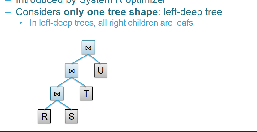
What are Left-Deep Join Trees?

To drastically reduce the number of possibilities, optimizers often restrict their search space exclusively to left-deep join trees.

• In a left-deep tree, every right-side child in the sequence is a base relation (a leaf) rather than an intermediate result.

• Benefits: These shapes generally yield excellent performance because they keep the "build" relation small, and they allow data to be continuously pipelined into the next operator without needing to write costly temporary result files to the disk.

• Even with this restriction, a 12-relation query still has 479 million possible left-deep combinations, meaning further optimization algorithms are required

What is Dynamic Programming?

Dynamic Programming is the traditional method used to find the optimal left-deep tree.

• How it works: It builds a table to systematically compute the cheapest cost for small subsets of relations (e.g., pairs of 2, then subsets of 3), combining them iteratively to find the best overall order.

• Pros: It guarantees finding the "best" join order based on the optimizer's cost estimations.

• Cons: It has an exponential complexity of O(2^n) and requires extra memory to store its cost tables. Because of this, it is only practically useful for queries containing up to 10-15 joins.

What is Greedy Join?

When a query is too large and dynamic programming becomes too expensive, optimizers switch to heuristic, greedy strategies.

• How it works: The algorithm simply looks at the available relations and starts by picking the single join pair that has the absolute cheapest cost (putting the smaller relation on the left). It then continuously attaches the next relation that promises the cheapest immediate join cost to the right side of the tree until all relations are joined.

• Trade-off: While this algorithm is incredibly fast at constructing a left-deep tree, it has a "myopic" view and is not guaranteed to find the globally optimal result.