Quantitative Measures of Psychology

population

set of all individuals of interest in a particular study

sample

set of individuals selected from a population, usually intended to represent the population in a study

populations are described using a…

parameter

samples are described using a

statistic

Descriptive Statistics

Techniques that allow us to describe a sample, often by summarizing information from individual observations

• Examples: frequency, mean, standard deviation

Inferential statistics

Techniques that allow us to use observations from a sample to make a generalization (i.e., inference) about the population from which that sample was drawn

• Examples: correlation, t-test, ANOVA, regression, chi-square

representative sample

sample whose distribution of varying characteristics matches that in the broader population of interest

Nominal

• use numbers only as labels for categories

• Order does not matter

• Qualitative/categorical

(what is your favorite form of exercise? running, walking, weightlifting, yoga? and you can assign a number to each form of exercise 1,2,3,4,5 but the greater values don’t mean anything)

Ordinal

• categories are ordered in terms of size or magnitude

• interval each category represents is not equal

• Order matters

  (How often do you exercise per month on a scale of 1-4? 1(never). 2(1-5 days), 3(6-10 days), 4(11 or more days) The difference between someone picking 1 and 2 is not equal amount of days compared to 2 and 3)

Interval

• Categories are ordered and represent roughly equal intervals

• no absolute zero point (since there is no absolute zero point, meaningful ratios can’t be calculated, you can only add or subtract interval data, not multiply or divide)

Example: Temperature, 0 degrees Celsius doesn’t mean there’s no temperature, it’s just another point on the scale (no absolute zero point)

Ratio

• Categories are ordered and represent roughly equal intervals

• True zero point (Since there is a true zero point, meaningful ratios can be calculated and you can add, subtract, multiply, divide)

  Example: A height of 0 cm means there is no height, this allows for meaningful ratios to be calculated because someone who reports being 6 feet tall is twice as tall as someone who is 3 feet tall.

central tendency

values where scores tend to center in a data set (mean, median, mode)

Mean

-average of scores

-sum of all scores divided by number of scores

limitations: sensitive to outliers

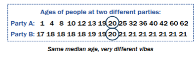
Median

-point that divides distribution in half

benefit: less affected by outliers

limitation: doesn’t utilize all scores; just based on rank order

Mode

-most frequently occurring score

limitations: like median, doesn't utilize all scores, and unclear to interpret if there's no mode

Nominal scale requires this kind of central tendency

Mode only

(because there are not really numbers so it only makes sense to see the most frequent point)

Ordinal scale requires this kind of central tendency

median and mode

(cant use mean because there are large spaces between ordinal data points and can throw it off like an outlier)

Interval and ratio scale requires this kind of central tendency

median, mean, mode

(there are equal spaces between data points in an interval scale so mean can be used)

operationalization

the process of defining how a variable can be measured, or the process of turning a conceptual variable into a measured variable

conceptual variable

abstract idea of interest in research

not always directly observable and/or might be observed multiple ways

measured variable

• concrete translation of the abstract idea into something that can be assessed quantitatively (often requires a thoughtful decision!)

• observable, empirical indicator

• what we typically examine with statistics

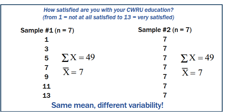
variability

the extent to which scores in a distribution differs from one another (dispersion, spread)

Measure of variability: range

highest score minus lowest score

shows how much spread there is from the lowest to the highest point in a distribution

Limitations: Doesn’t utilize all scores (just the lowest and the highest affects it) ; may be inflated by outliers

Alternative to range: interquartile range - range of the middle 50% of scores (not affected by extreme values)

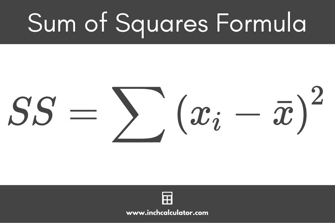
Measures of variability: Sum of squares

Sum of squared deviations from the mean

If SS is 0, all the data is the same, no deviation from the mean (no variability)

SS cant be negative because the values are squared

Limitations:

-values are in squared units (not the original response scale)

-tied to sample size (more responses by people/sample = more deviations in the sum)

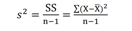
Measures of variability: variance

average squared deviation from the mean

Drawback: Still in squared units, still tricky to interpret

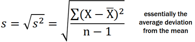
Measures of variability: standard deviation

square root of the variance

The average distance of each score from the mean. The larger the standard deviation, the more spread out the values are, and the more different they are from one another.

Drawbacks; sensitive to extreme scores

Benefits: the standard deviation is stated in the original units it was derived

Measures of variability

• provide information about how scores in a distribution differ from one another

▪ Variability can be in terms of ranges of scores...

▪ Or in terms of how much scores differ from the sample mean (sum of squares, variance, and standard deviation)

▪ Each measure of variability conveys different, but useful, information

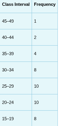
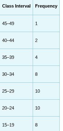
Frequency Distribution

A method of tallying and representing how often certain scores occur. Scores are usually grouped into class intervals, or ranges of numbers.

the distribution of frequencies for each level of a given variable observed in a sample (or population) and representations thereof

• Or how all X’s in a given sample were distributed across the different categories/scores/etc. for a variable

class interval

a range of numbers

1. Select a class interval that has a range of 2, 5, 10, 15, or 20 data points. In our example, we chose 5.

2. Select a class interval so that 10 to 20 such intervals cover the entire range of data. A convenient way to do this is to compute the range and then divide by a number that represents the number of intervals you want to use (between 10 and 20). In our example, there are 50 scores, and we wanted 10 intervals: 50/10 = 5, which is the size of each class interval. If you had a set of scores ranging from 100 to 400, you could start with an estimate of 20 intervals and see if the interval range makes sense for your data: 300/20 = 15, so 15 would be the class interval.

3. Begin listing the class interval with a multiple of that interval. In our frequency distribution of reading comprehension test scores, the class interval is 5, and we started the lowest class interval at 0.

4. Finally, the interval made up of the largest scores goes at the top of the frequency distribution.

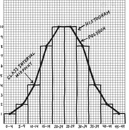
histogram

a visual representation of the frequency distribution where the frequencies are represented by bars.

Frequency Polygon

A continuous line that represents the frequencies of scores within a class interval.

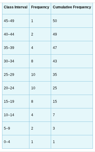
cumulative frequency distribution

The cumulative frequency distribution begins with the creation of a new column labeled “Cumulative Frequency.” Then, we add the frequency in a class interval to all the frequencies below it. For example, for the class interval of 0–4, there is 1 occurrence and none below it, so the cumulative frequency is 1. For the class interval of 5–9, there are 2 occurrences in that class interval and one below it for a total of 3 (2 + 1) occurrences. The last class interval (45–49) contains 1 occurrence, and there are now a total of 50 occurrences at or below that class interval.

Benefits of tables and graphs

Benefits to researcher

• How do your data (literally look), descriptively? What did your sample give you?

• Identifying outliers and extreme scores

• Identifying floor or ceiling effects

  -When a large potion (around 75%) of your sample is at the bottom/top of the possible response distribution

Benefits to your audience?

• Helps them make sense of what you found

Frequency Tables

• Report the distribution of frequencies in table form

  -(f) frequency

  -(rf) relative frequency, ratio or proportion of this response in the sample (f/n) = rf

  -percentage of this response in the sample (rf x 100%) = %

• (cf) - cumulative frequency - adding what’s at or below that level for each level starting at the bottom of the scale

  -(crf) cumulative relative frequency - successive total of relative frequencies (often from bottom value) cf/n = c%

• (c%) - cumulative percentage - successive total of percentages (often from bottom value)

frequency alone can be misleading because it doesn't account for the total people in a sample, that's why relative and percentage is important. (i.e 75 dentists recommend a certain kind of brush, but it’s 75 out of 1000 dentists who were asked)

Frequency Graphs

Report the distribution of frequencies in visual form

• Bar graph (appropriate for nominal data)

• frequency histogram (appropriate for data with a limited range of possible values)

• frequency histogram with class intervals (appropriate for data with many possible values)

• frequency polygon (appropriate for data with many possible values)

  • line graph with points that represent class interval frequencies

Guidelines for good tables and graphs

• Think about what you most want to communicate about your data in a straightforward way

  - Report a simple, manageable amount of information

• Dont include tables and graphs that aren’t useful to audience

Label everything clearly

For graphs:

• Axis scales should make sense and have uniform units; if you don’t start at 0 include a hash mark to indicated a break

• Y- axis should be 2/3-3/4 length of the x axis

Sampling Error

No single sample will ever completely and accurately describe a population of which that sample was taken from, it is the natural random difference between a sample result and the true population value.

Unbiased Estimate

• Statistic whose average across all possible random samples of a given size equals the parameter (μ)

• Some X̄ will overestimate μ some will underestimate μ but the mean of X̄s across all possible samples of a given size will equal μ

• sample mean X̄, is considered an unbiased estimate of population mean μ

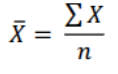
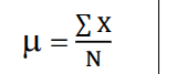
Population Parameter Mean

μ = ΣX / N

N = number of X’s in the population

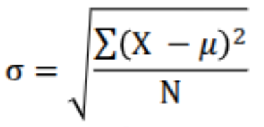
Population Parameter Standard Deviation

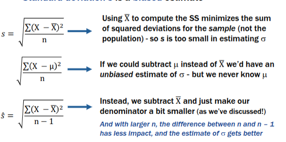
Sample Estimate of Parameter - Mean & Standard Deviation

• sample mean X̄, is considered an unbiased estimate of population mean μ

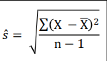
• The adjusted sample standard deviation (ŝ), based on n - 1, not n to reduce bias in its estimation of population standard deviation (σ)

Which statistic is not an acceptable estimate?

Standard Deviation or s, is a biased estimate

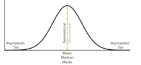
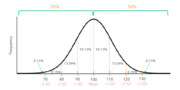
Normal Distribution, Normal Curve, Bell Curve

• is a visual depiction of a distribution of scores

• is characterized by an identical mean, median, and mode; symmetrical halves; and asymptotic tails.

• can be divided into sections with corresponding probabilities.

• can be used to assess the probability of an event occurring.

The Empirical Rule (Normal Distribution)

• 68% of the data falls within 1 standard deviation of the mean

• 95% of the data falls within 2 standard deviations of the mean

• 99.7% of the data falls within 3 standard deviations of the mean

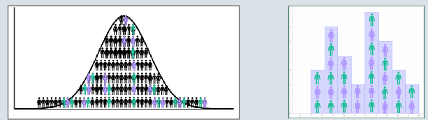
Why are many variables normally distributed?

1. Each case/event that represents one data point of the distribution is affected by numerous random factors

2. Some random factors push values above the mean, while others push values below the mean

3. When combining the influence of random factors, scores close to the mean/median are the most common

4. Extreme scores are unlikely– few cases have ALL variables strongly pushing in the same direction

If a population distribution is normal, will the sample distribution be normal?

Yes if population dis. is normal then any random sample you draw will also be normal because when the population is normal, the subset/samples tend to follow the same shape as the population.

If a sample dis. is normal, does that mean the population dis. is normal?

No because a small sample can appear normal even if the population distribution is skewed or has heavy tails, in order to infer population normality you’d need multiple samples and larger sample sizes or additional statistical tests.

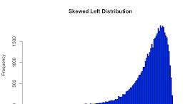
Left/ Negative Skew

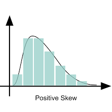
Right/ Positive Skew

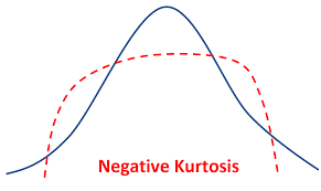
Platykurtic Kurtosis

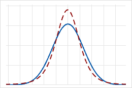
Leptokurtic / Positive Kurtosis

If your distribution isn’t normal then..

DO:

• Look into non-parametric tests because they don’t assume normality and are safer for irregular/skewed data

• Consider how expected population characteristics, sampling methods, and measures may have influenced your sample distribution. (i.e small sample, naturally skewed population, etc)

DON”T:

• Make inferences about the distribution of population scores based on the Empirical rule because it only applies to normal distributions.

• Don’t use common statistical tests that assume normality such as t-tests, ANOVA, etc

What are z scores/standard scores drawn from?

Any specific distribution of scores, based on that specific distribution’s mean and standard deviation

What do z/standard scores represent?

“Standardized” scores that reflect how many standard deviations each observation is from the mean of the distribution

What do standard scores/ z scores help us to do?

• Quickly grasp where a specific observation falls within its distribution

• Compare observations from different distributions

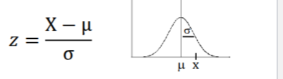
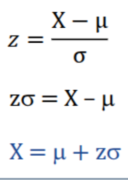
Population z score formula

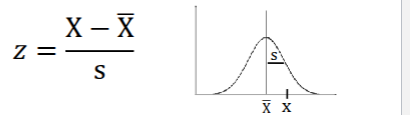
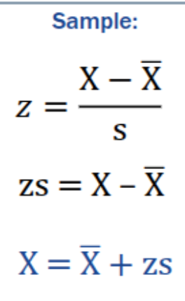
Sample z score formula

The equation for transforming a z score to a raw score (population)

The equation for transforming a z score to a raw score (sample)

interpreting Standard Scores

• absolute value of the z score = number of standard deviations X is from the mean

• positive z score = X is above the mean

• negative z score = X is below the mean

• If a z score is 0 then X is at the mean because mean = 0

• If z score is 1 then X is exactly one standard deviation from the mean because S.D = 1

• Most values fall between positive/negative 3 standard deviations because of the empirical Rule which states that about 99.7% of data of values in a normal distribution fall within 3 standard deviations from the mean

• A skewed distribution that gets standardized will still be skewed when it gets standardized 

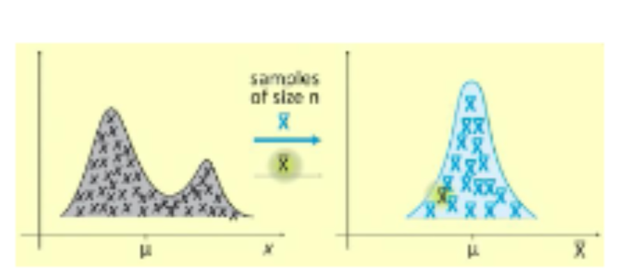
Sampling distribution of the mean

= the theoretical distribution of mean scores from all possible samples of a given size within a population (I.e frequency distribution of X̄ for all possible samples of n size)

Example: I

• The center of the distribution will be population mean (μ) Even though the the means of individual samples differ, the average of all the sample means equals the true population mean (μ)

• Allows us to conceptualize variability in sampling error in estimating μ across different samples of a given size. In other words, the distribution helps us to see how much sample means tend to vary from sample to sample

Central-Limit Theorem

• Describes the sampling distribution of the mean for any given population with mean (μ) and standard deviation sigma (σ)

• This theorem states that if you take many random samples from any population (normal or not), and compute the means the sample means will..

1. Center around the true population mean (μ)

2. Have a predictable spread (standard error)

3. Form a normal-shaped distribution (as long as the sample size (n) is large enough ~30+

Is each sample statistic a perfect estimate of the population parameter?

No, every sample you take will be a little different from the population as a whole, and that difference is called sampling error. Every sample statistic has some error, but if you average across many random samples, the sample mean is still a good estimate of the population mean. 

Sampling Distribution of the mean Equations

For any given sampling distribution of the mean…

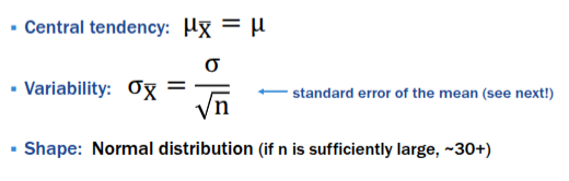
• Central tendency: 𝜇X̄ = 𝜇

- The mean of all the sample means equals the true population mean. Sample means are unbiased estimates of 𝜇

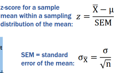
• Variability: σX̄ = σ / (n)^1/2

- This is called the standard error of the mean, it tells us how much sample means vary from sample to sample. As sample size (n) increases, the standard error of the mean becomes smaller. 

- Larger samples —> less variability —> more precise estimates 

• Shape

-The distribution of sample means will be approximately normal is n is large enough

-Even if the population isn’t normal (ex: skewed) the distribution of sample means distributes itself normally as n gets larger

Limits of Sample Statistics

• We can never be certain that our sample statistics are a perfect match to the population parameters they estimate because of sampling error (every sample is a little different)

- However, larger samples tend to offer better estimates

• If we could collect all possible samples of n size in a population, the

distribution of their means is the sampling distribution of the mean

 -Its mean is 𝜇; its standard deviation is called the standard error of the mean

 -Bigger samples will lead to a sampling distribution of the mean with a smaller standard error of the mean

▪ We must always keep in mind that what we find for any given sample may not match what is true in the population

   -However, we can use inferential statistics to see if we have reason to believe that is not the case

Forming/ Identifying a research question (Step 1)

• Identify variables of interest (an element in research that can vary)

• Ask about systematic associations and/or differences that exist among these variables (e.g Is there an association between [variable 1] and [variable 2]?) or “Do people with [a level of variable one] differ from those with [another level of variable 1] in [variable 2]?”

 State Hypotheses (Null Hypothesis (H₀)) (Step 2)

A statement of no relationship between variables and/or no difference in values

(i.e statement of equality or a lack of association)

• There is no association between these variables. These groups do not differ [are the same] on this variable

• Null hypotheses is our default! We assume variables are unrelated in this population unless we have evidence to suggest otherwise

Purpose: allows researchers to avoid making false assumptions about what’s true/not true in the population so it’s safe to assume that there no associations between variables unless research proves otherwise

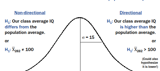
State Hypotheses (Research Hypothesis (H₁)) (Step 2)

A statement that a relationship exists between variables and/or values differ

• i.e (a statement of inequality or association)

• Also called an alternative hypothesis (I.e alternative to H₀) 

        - Non-directional hypothesis: a relationship or difference exists among variables (“two-tailed test,” could go either way)

       -Directional hypothesis: a specific direction of relationship or difference exists (“one-tailed tests”)

Process for hypothesis testing

1. identify research question

2. State null hypothesis and research (alternative) hypothesis

3. Define statistical significance

4. Conduct an inferential statistical test

5. Reject (or fail to reject) the null hypothesis

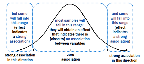
Defining Statistical Significance (Step 3)

We can never be certain that a strong association between variables found in one sample isn’t just an extreme case in a population for whom H₀ is nonetheless true

• Every sample could be a fluke it in its population (sampling error)!

▪ So, we must decide how much of a chance we are willing to take, or what effect we think is extreme enough to indicate that H₀ may not be true in the population

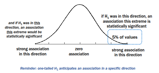
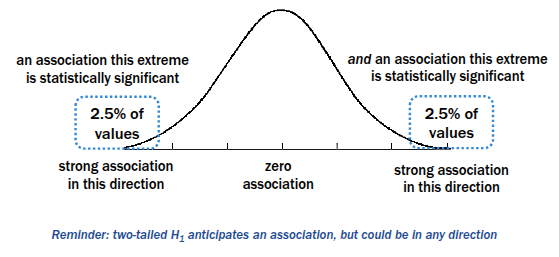
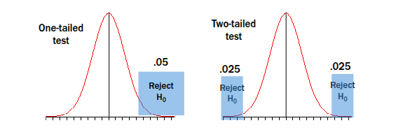
▪ Statisticians have agreed on a critical value of <.05

• We agree that an effect we would find less than 5% of the time if H₀ was true is statistically significant

if H₀ is true..

If H₁ is true (One-Tailed Hypothesis)

if H₁ is true (Two-Tailed Hypothesis)

Conducting a inferential statistical test (Step 4)

• Every null hypothesis (H₀) can be tested with an inferential statistic (like a t-test, z-test, ANOVA, etc)

• A statistical test yields:

      -Test Statistic —> a numerical value that represents the strength of the effect in your sample (e.g. a t-value)

      --p-value —-> the probability of getting a result this extreme if H₀ is true

• If p is less than 5% or 0.05 it means that such a result would only happen less than 5% of the time by chance, making it statistically significant 

Rejecting the null hypothesis (Step 5)

• If your inferential statistic has a p-value less than .05, you may reject the null hypothesis

• The effect you obtained is extreme enough to suggest that H₀ is not true in the population

Failing to Reject Null Hypothesis (Step 5)

• Null Hypothesis (H₀): assumes no effect, no difference, or no association

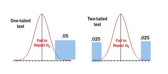
• Fail to Reject H₀: your result is not rare/extreme enough to reject the null.

• Fail to reject the null does not mean proving the null, it just means no strong evidence against it.

If most results fall in the middle of the graph  (common results) —> p is larger than 5% —> fail to reject H₀

Interpreting and Phrasing Conclusions (Step 5)

Remember that p < .05 is:

-an agreed-upon critical value for rejecting H₀, not the law

-a value associated with sample data, not conclusive evidence about what is true in the population

Be careful with how you interpret (and phrase) your conclusions!

• You may reject H₀ based on sample data, but that doesn’t mean you accept H₁ (or that you have proven H₁)

• We may fail to reject H₀ based on sample data, but that doesn’t mean we accept H₀ (or reject H₁, or have disproven H₁)

Z-Test

• The appropriate inferential statistic to compare a sample mean to a given population mean is a one-sample z-test

• z tests are difficult to use because we rarely know μ in actual research samples!

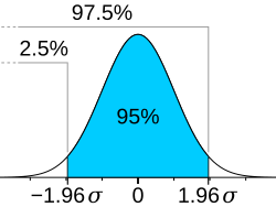
• Since positive 1.96 z-score and negative 1.96 z-score add up to 95%, any z-score that is greater than + or - 1.96, is less than 5% making it statistically significant 

Type I Error (α-alpha)

Saying there is an effect when there isn’t aka rejecting the null, when the null is actually true 

Type II Error (β-beta)

Saying there’s no effect when there actually is, failing to reject the null when the null is false

Power

The probability of correctly rejecting H₀ when H₀ is false, or the probability of detecting an effect that really exists in the population.

= 1 - β

What affects power?

• the alpha level you set (typical α  = .05)

• A higher alpha level —> easier to reject H₀ —> increases power (but also increases Type I Error risk)

• sample size & variability of samples

• larger sample size —> less random noise —> increases power

• less variability —> clearer signal —> higher power

• actual size of the effect in the population

• Larger, real effects are easier to detect —> higher power and vice versa

Bottom Line: High power means your study is good at finding real effects and avoiding false negatives (Type II Errors) 

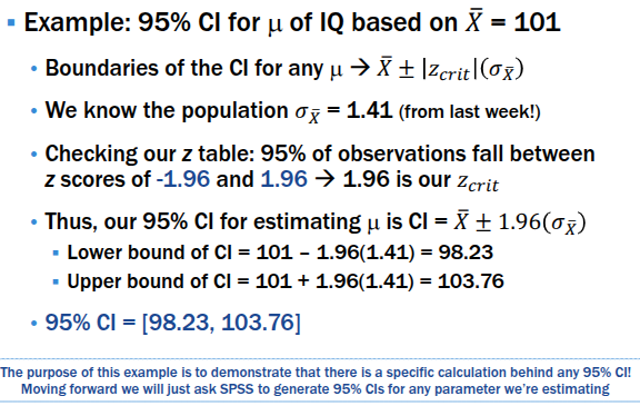
Confidence Intervals

• A test statistic (like a sample mean) is only one estimate of the true population parameter.

• It’s an imperfect estimate because there’s uncertainty in how well it represents the population.

Confidence Intervals: - estimated interval of values you have __% confidence contains the actual population parameter

• 95% confidence interval is the most common 

• In a 95% Confidence Interval, it is 95% certain that the actual population parameter falls within the range of values in this interval

Confidence Interval Example

Confidence Intervals In Hypothesis Testing

• Often a value of 0 for an inferential statistic indicates zero effect (no difference, no association, etc.)

• In that case, we test a H₀ that the population parameter = 0

1. If the 95% Confidence Interval for a population parameter includes 0,

•  Corresponds with p > .05 

• Conclusion: Fail to reject H₀ 

2. If the 95% Confidence Interval for a population parameter does not include 0, it means the estimate is far enough from 0 that it’s statistically significant.

• Corresponds with p < .05 

▪ Conclusion: Reject H₀ 

Confidence Intervals In Hypothesis Testing Example

Suppose you calculate a 95% CI for the mean difference between two groups:

CI = [2, 6]

This means we’re 95% confident the true difference is somewhere between 2 and 6.

👉 Notice that 0 is not inside this range. That means 0 (no difference) is not a plausible value.

Conclusion: Reject H₀

Another example:

CI = [-3, 4]

This means we’re 95% confident the true difference is somewhere between -3 and 4.

👉 Notice that 0 is inside this range. That means it’s plausible that the true difference is 0 (no difference)

Conclusion: Fail to reject H₀

Making Causal Inferences

1. Before we move forward with specific statistical tests, we should keep in mind:

 - Rejecting H₀ means you may reject the default assumption that your variables are not associated, based on your sample data

 - However, this does not mean you can conclude these variables are causally associated, i.e., variability in one causes variability in the other

Experimental Research Design 

▪ The only design that allows for a test of causal relationships

• Identify an independent variable and dependent variable

• Manipulate the IV (i.e., assign participants to different groups/levels of your IV), keep everything else the same for participants, then measure the DV

• Internal control like this allows you to infer that any variation in the DV was caused by variation in the IV

Correlational Research Design 

• Tests associations between variables, but cannot assume they are causal

• Measure variables as they exist, no manipulation involved

▪ Often because it is impossible and/or unethical to do so

• Without experimental control, you can find a statistical association between the variables, but cannot infer it is causal

• Confounding Variable: A confounder is a hidden variable that muddies the results by creating false association or masking a real one

Examples of Confounding Variables:

False association: People who carry lighters seem more likely to get lung cancer, but the confounder is smoking—it causes both.

Masking a real association: Exercise lowers blood pressure, but if you don’t account for age (older people exercise less and have higher BP), the effect looks weaker.

Both experimental and correlational studies can…

examine variables at any level of measurement

• Nominal data do not imply control vs. experimental group

• Ordinal/interval/ratio data do not imply a lack of manipulation

▪ Thus, the appropriate inferential statistical test for a study is based on the amount of variables being tested and their measurement scales

• Doesn’t prove cause and effect 

Correlations between variables

A correlation coefficient (r) represents a linear association between two variables (X and Y) measured in the same people

• May view one variables as IV/predictor and other as DV/outcome, or just two variables that may be related

Variables are on  an interval or ratio scale (ordinal with caution)

• continuous scale reflecting different magnitudes of this variable; scores reflect a range from lower to higher values

Variables are between-subjects

• every person has only one value of each variable along its range

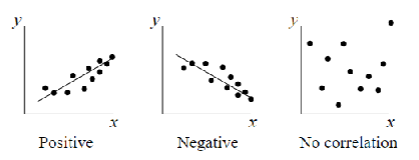
Characteristics of a correlation between X and Y

• Direction of association

• Magnitude of strength of association 

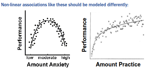
• Type of association: assumed to be linear

Direction (Characteristics of a Correlation)

• Positive - higher value of X relates to higher values of Y (or lower value of X relates to lower value of Y)

• Negative (inverse) - higher values of X relates to lower value of Y (or lower value 0f X related to higher values of Y)

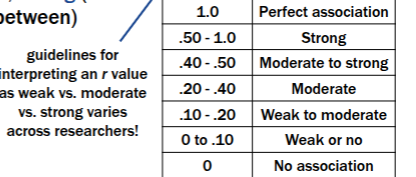
Magnitude (Characteristics of a Correlation)

• Absolute value of 0 to 1, reflecting degree of linear fit

• Combined with direction to range from -1.00 to 1.00

• Typically described as weak, moderate, strong (or somewhere in between)

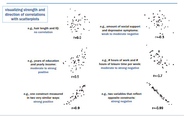
Correlation Scatterplot Examples

Type of Association (Characteristics of a Correlation)

• X and Y must have a linear association for a correlation coefficient to be an appropriate fit

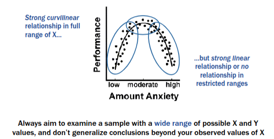
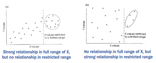
Potential issues fitting a correlation to sample data - Restricted Range of Data

- Observing only limited variation in X and/or Y in a sample can misrepresent their correlation in the population

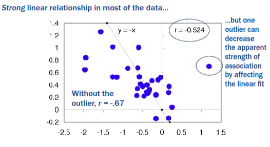
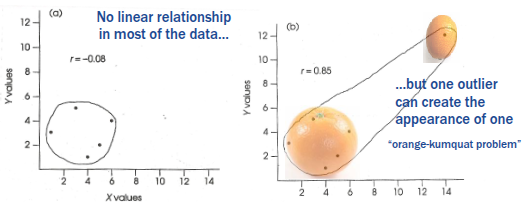
Potential issues fitting a correlation to sample data - Outliers

-  May completely change the apparent fit of a linear association within the data

- May lead one to misrepresent the correlation that actually exists in most of the sample data and/or the population

Left graph:

Most of the data points show no real linear relationship (correlation close to 0, r =  - 0.08).

Right graph:

Adding a single outlier far away from the rest of the data suddenly creates the illusion of a strong positive correlation (r = 0.85).

→ This is called the “orange–kumquat problem”: the outlier is so different that it falsely drives the correlation.

Key point:

Outliers can completely change the correlation coefficient (r) and make it look like there’s a strong relationship when there really isn’t.

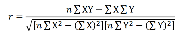
Pearson product-moment correlation (r)

▪ Most commonly-used inferential statistic for a zero-order correlation (i.e., a simple correlation between two variables)

▪ Conceptually, reflects the position of any score in the X distribution (relative to its mean) and the corresponding position of a score in the Y distribution (relative to its mean)

• Like a calculation of how z scores for X and z scores for Y vary together across the sample

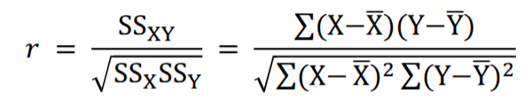
Pearson product-moment correlation (r) Definitional Formula

As before, SS = sum of squares, reflects how much a set of scores varies from its mean; here we have SS_X for variable X and SS_Y for variable Y.

SCP = SS_XY – reflects how much 2 sets of scores (X and Y) vary together, i.e., covary

Computational formula for r

• draws out elements of the definitional formula to allow for a more straightforward calculation