wk2 - probability and parameter estimation

posterior probabilities

probability of the class after observing the data (evidence)

prior

probability of the class before observing the data (evidence)

likelihood

probability of observing a random data point given the class label (compatibility of the data with the given class)

evidence

probability of observing a (random) data point across all classes

Bayes Decision Rule

P(x|w1)P(w1) > P(x|w2)P(w2)

continuous random variable

a variable that cam take any value within a range (interval of real numbers)

- they are not countable

- they are measured not counted

what is the probability that a continuous random variable is equal to a specific value? P(X=x)

around 0, infinitely small

uniform distribution

every value within the range (a,b) is equally likely. therefore the probability density has a constant height of (1 / b-a)

total area under should equal 1

triangle distribution

the height of the triangle is chosen as (2 / b-a) with the total area being (base x height / 2)

univariate gaussian distribution

parameter μ controls location of the peak

parameter σ controls the width of the peak

defined for the range (-infinity < x < infinity)

also called the normal distribution

F(x) = P(X <= x)

cumulative distribution function

properties of the PDF

1. its values cannot be negative

p(x) >= 0 for all x

2. the area under the curve must equal to 1

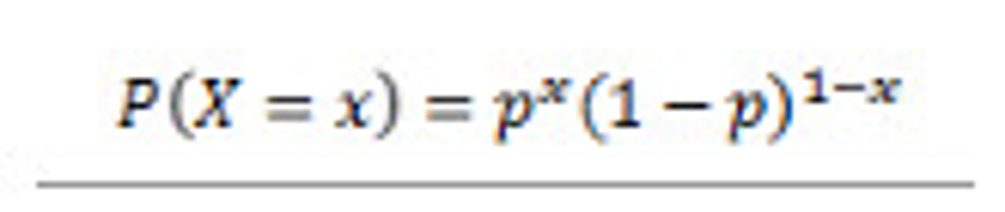
bernoulli distribution

discrete probability distribution that models a random variable which takes only two possible outcomes (success / failure)

how are sample data stored in a matrix

each sample x is formulates as a N by L matrix, having N samples (rows) and L features (columns)

so each row is a sample, and how many columns is how many features it has

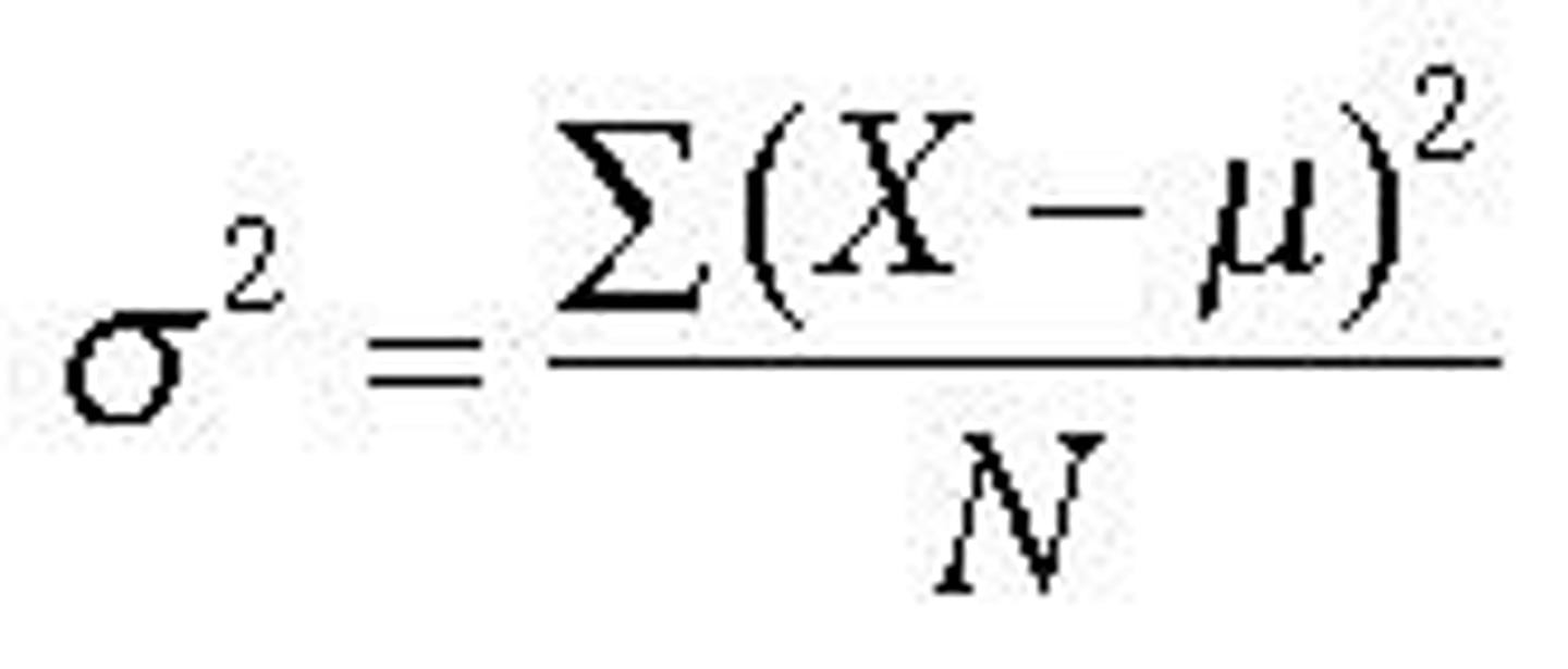
variance

this measures the spread of the data

to calculate this

you take away the mean from the sample, then square the result. do this for every one and then divide by how many you just did

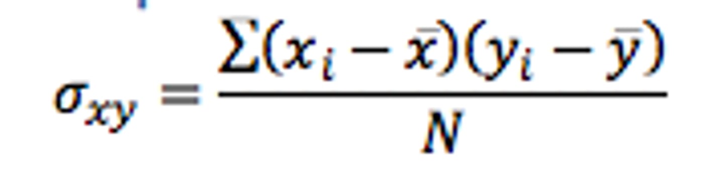
covariance

measure of association / correlation between two variables. it describes how the two variables relate or change together

times together the difference between sample and mean for two different variables for every one in the sample and divide by however many.

if both tend to increase or decrease togetherm then the covariance is positive

if one increases while the other decreasesm the covariance is negative

if they are independent, the covariance is closer to zero.

covariance matrix

the diagonal elements are the variances

the off-diagonals are the covariances

population statistics

refers to the entire group of data points that we are interested in studying. e.g. all adults in the UK.

population parameters are the true but usually unknown values that describe the population

sample statistic

a subset of the population selected for analysis

used to estimate population parameters

sample mean

unbiased estimate of the population mean

sample covariance

biased estimate of the population covariance

unbiased estimate of the population covariance

( N / (N-1) ) S

parameter likelihood function

it expresses the probability of observing the given data (random samples) as a function of the parameters θ

think of it as the probability that all the datapoints came from the distribution with parameters θ

maximum likelihood estimate (MLE)

estimates the parameters θ that best maximise the likelihood based on the data

why do the maximum likelihood estimate?

this function is to estimate the parameters θ that make the observed data most probable. by maximising the likelihood function p(X;θ), we find the parameter values that best explain the observed data.

what does sample independence mean for the likelihood function

we can factorise the probabilities.

product operator

used to represent a product of the sequence (just times everything together)

how to find the MLE

we need to find the values of θ where

∂p(X; θ) / ∂θ = 0

the gradient of the likelihood is zero when θ = MLE

log likelihood

this is easier

L(θ) = ln p(X; θ)