3 Decision tree

R & C

Decision Tree

Decision trees split data into branches based on feature values, creating decision nodes until reaching final predictions. A decision tree is a supervised learning algorithm for classification and regression tasks. It represents decisions and their possible outcomes in a tree-like structure, making the decision-making process transparent and interpretable.

pruning in the context of decision trees

Pruning is a technique used to reduce the complexity of a decision tree by removing unnecessary branches.

It aims to: Reduce overfitting. Improve model generalization on unseen data.

Two common types are: Pre-pruning: Stops tree growth early based on criteria (e.g., depth, minimum samples).

1. Post-pruning: Removes branches from a fully grown tree using validation data.

2. Pruning ensures that the tree remains interpretable and avoids capturing noise in the training data

Root Node

The decision-making process starts at the root node, representing the entire dataset. The model evaluates the best feature to split the data based on a chosen criterion like Gini Impurity, Information Gain (for classification), or Mean Squared Error (for regression).

How do we find the root node

1. Calculate Impurity/Information Gain:

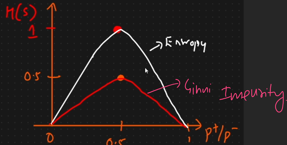
   • Gini Index: Measures impurity. Lower values are better.

   • Entropy: Measures disorder. Higher information gain is better.

2. Evaluate Each Feature:

   • For each feature, calculate the Gini Index or Entropy for all possible splits.

   • Determine the information gain for each split.

3. Select the Best Feature:

   • Choose the feature with the lowest Gini Index or highest information gain.

   • This feature becomes the root node.

Splitting

The dataset is divided into subsets based on the selected feature's values, creating branches from the root node. This process continues recursively at each subsequent node.

Internal Node

These nodes represent decision points where the dataset is further split based on other features.

Leaf Node

These are terminal nodes that provide the final prediction.

For classification tasks, the leaf nodes contain class labels, while for regression tasks, they provide numerical outputs.

Stopping Criteria:

All data points in a node belong to the same class (pure node).

■ A maximum tree depth is reached.

■ Minimum samples per leaf or minimum information gain criteria are met.

How do we split

• Entropy

• Ginny Index

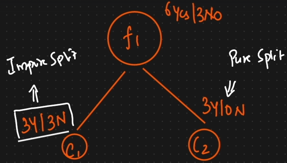
Pure split vs Impure split

pure if all the resulting child nodes contain instances of only one class.

impure if the resulting child nodes contain a mix of different classes.

For huge data set we will use what split method

Gin Impurity (Categorical Feature)

problem with the decison tree

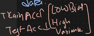
This will cause overfitting of data.

How do we reduce the overfittig of data

• Post Pruning

• Pre Pruning

Post Prunning

we will complete decision tree an later we will cut that (Pruning).

For smaller data we will use ____ Prunning

Post

Pre Pruning

we will use some parameters while construction of parameters.(max feature, Depth ,max depth, Split )

For huge data we will use

Pre Pruning

How does a Random Forest algorithm work?

Random Forest is an ensemble learning method that combines multiple decision trees to improve predictive performance.

1.Bootstrap Sampling: Random subsets of the data are created (with replacement)

2.Tree Construction: Each tree is built independently using a subset of features.

3.Aggregation: For classification, predictions are based on majority voting. For regression, predictions are averaged.

This approach reduces overfitting and increases robustness, making it suitable for high-dimensional data.

Decision Tree vs Random Forest

Feature	Decision Tree	Random Forest
Algorithm Type	Single tree-based model	Ensemble of multiple decision trees
Overfitting	Prone to overfitting	Less prone to overfitting due to averaging
Bias-Variance Tradeoff	High variance, low bias	Lower variance, slightly higher bias
Interpretability	Easy to interpret and visualize	Harder to interpret due to multiple trees
Training Time	Faster training time	Slower training time due to multiple trees
Prediction Time	Faster prediction time	Slower prediction time due to averaging predictions
Accuracy	Can be less accurate due to overfitting	Generally more accurate due to ensemble approach

How do we select feature

Using entropy (measure the randomness of a system)

Gini Index vs Entropy

Aspect	Gini Index	Entropy
Definition	Measures the impurity or impurity of a dataset.	Measures the disorder or uncertainty in a dataset.
Formula	Gini=1−∑i=1npi2Gini=1−∑i=1n​pi2​	Entropy=−∑i=1npilog⁡2(pi)Entropy=−∑i=1n​pi​log2​(pi​)
Range	0 (pure) to 0.5 (maximum impurity for binary classification)	0 (pure) to 1 (maximum disorder for binary classification)
Interpretation	Lower values indicate purer nodes.	Higher values indicate more disorder.
Calculation Complexity	Simpler and faster to compute.	More complex and computationally intensive.
Usage in Decision Trees	Often preferred due to computational efficiency.	Provides more information gain but is computationally heavier.
Sensitivity to Changes	Less sensitive to changes in the dataset.	More sensitive to changes in the dataset.

TYPES of Decision trees - CART vs C4.5 vs ID3

Aspect	CART	C4.5	ID3
Splitting Criterion	Gini Index	Information Gain Ratio	Information Gain
Tree Structure	Binary trees (two children per node)	Multi-way trees (multiple children per node)	Multi-way trees (multiple children per node)
Data Types	Continuous and categorical	Continuous and categorical	Categorical only
Pruning	Cost-complexity pruning	Error-based pruning	No pruning
Handling Missing Values	Surrogate splits	Assigns probabilities	Does not handle missing values
Advantages	Simple, fast, easy to interpret	Handles both data types, robust pruning	Simple, easy to understand
Disadvantages	Can overfit without pruning	More complex, computationally intensive	Can overfit, does not handle continuous data

Do we require Scaling ?

Tree-based Algorithms: Algorithms like Decision Trees and Random Forests don't need scaling because they split data based on feature values, not distances.

How Does the Decision Tree Algorithm Work for Classification in Machine Learning?

A Decision Tree is a supervised machine learning algorithm used for classification and regression tasks. It works by splitting the dataset into smaller subsets based on feature values, forming a tree-like structure.

Select the Best Feature (Splitting Criterion):

The algorithm chooses the feature that best separates the data using criteria like Gini Impurity, Entropy, or Information Gain (in ID3, C4.5, or CART algorithms).

Split the Dataset:

Based on the selected feature, the data is split into branches.

Each branch represents a possible decision or outcome.

Repeat Recursively:

The process continues recursively on each subset until one of the stopping conditions is met:

All data points in a node belong to the same class.

The maximum tree depth is reached.

The information gain from further splits is too small

Make Predictions: Once the tree is built, new data points are classified by following the decision paths from the root to a leaf node, where a class label is assigned.

How Does Gradient Boosted Decision Trees (GBDT)Differ from Random Forests?

Gradient Boosted Decision Trees (GBDT):

An ensemble method where trees are builtsequentially. Each tree attempts to correct the errors ofthe previous one. The focus is on minimizing a lossfunction (e.g., mean squared error) through gradientdescent.

Advantages: Strong predictive performance, especiallyfor structured data, and can handle different types ofloss functions.

Random Forests:

An ensemble method that builds multiple decisiontrees in parallel, each trained on a random subset of the data with random feature selection for splittingnodes.

Advantages: More robust to overfitting than a singledecision tree and generally faster to train than GBDT.

GBDT usually performs better in terms of accuracy but is slower and more prone to overfitting if not tuned properly,while Random Forests are easier to train and tune.

What distinguishes a poorly performing classifier(a "bad classifier") from a Random Forest model,and how do their design and performancecharacteristics differ in practice?

A "bad classifier" typically refers to a model thatunderperforms due to flaws like high bias/variance, poorgeneralization, or unsuitability for the data (e.g., linearmodels for non-linear problems). Random Forest, anensemble of decision trees, addresses many of theseweaknesses:

1.Model Complexity :

a. Bad Classifier: Often overly simplistic (e.g., a singleshallow decision tree) or overly complex (e.g., an overfitneural network) for the task.

2.Overfitting:a. Bad Classifier:

Prone to overfitting (e.g., a deep,unpruned decision tree) or underfitting (e.g., a linearmodel on non-linear data).

b. Random Forest: Mitigates overfitting by averagingpredictions across diverse trees trained on randomsubsets of data/features.

3.Feature Interactions:

a. Bad Classifier: May ignore complex feature relationships(e.g., logistic regression).

b. Random Forest: Automatically captures non-linearinteractions and hierarchies through split decisions inmultiple trees.

4.Robustness:

a Bad Classifier: Sensitive to noise, outliers, or irrelevantfeatures (e.g., k-NN without scaling).

b. Random Forest: Robust to noise and outliers due tomajority voting and feature subsampling.

5.Interpretability:

a. Bad Classifier: Sometimes overly interpretable butineffective (e.g., Naive Bayes with violated assumptions).

b. Random Forest: Less interpretable than single trees butprovides feature importance scores for insights.

6.Scalability:

a. Bad Classifier: May scale poorly (e.g., SVM with large datasets).

b. Random Forest: Parallelizable and efficient for medium-large datasets, though slower than gradient-boosted trees.

How Do Partial Dependence Plots Help InterpretMachine Learning Models?

Partial Dependence Plots (PDPs) visualize the relationshipbetween a feature and the predicted outcome, whilekeeping other features constant.

Function:

PDPs help interpret the impact of a singlefeature or a pair of features on the model’s prediction.

Use: These plots show whether a feature has a linear,non-linear, or no significant effect on the targetvariable, aiding in model interpretability by highlightingthe influence of individual predictors