The Phillips Curve

Who was Bill Phillips?

A renowned New Zealand economist and professor at the London School of Economics (LSE), best known for creating the "Phillips Curve" in 1958, which established the inverse relationship between unemployment and inflation.

What does the Phillips curve show?

A correlation between the rate of change of money wages and the unemployment rate.

Why have economists equated wage inflation with price inflation?

This is because changes in money wages are a key component of changes in prices. For most firms, wages and salaries are a significant proportion of their total costs and if wages rise than so do prices.

The Phillips Curve diagram

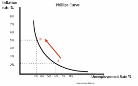
What does the Phillips curve suggest?

That changes in the level of unemployment have a direct and predictable effect on the level of price inflation.

Higher AD and the Phillips curve

Expansionary fiscal policy (↑G / ↓T) increases AD → firms raise output → higher demand for labour → unemployment falls (e.g. 5% → 3%).
Increased demand for factors of production raises wages and costs → firms raise prices → higher inflation (e.g. 6%).

Lower AD and the Phillips curve

Deflationary fiscal policy (↓G / ↑T) reduces AD → spending falls → firms cut output → lower demand for labour → unemployment rises (e.g. 3% → 5%).
Reduced demand for factors of production lowers wages and costs → firms cut prices to boost demand → inflation falls (e.g. to 2%).

How have governments exploited the Phillips curve?

Policy-makers believed there was a stable trade-off between inflation and unemployment, allowing them to choose a preferred combination.
To cut unemployment (e.g. 5% → 3%), governments boosted AD and accepted higher inflation (e.g. 6%).
In the 1960s–70s, governments used stop–go policies—expanding or contracting the economy via fiscal policy—to target desired inflation or unemployment rates.

What did the ‘GO’ phase refer to?

Boost AD to create growth and reduce unemployment, BUT this led to demand pull inflation and a trade deficit.

What did the ‘STOP’ phase refer to?

Cut to AD to decrease inflation and the size of the trade deficit, BUT this led to increased unemployment and slower growth.

The breakdown of the Phillips curve

By the mid-1970s the stable Phillips Curve trade-off broke down: economies experienced stagflation—high inflation alongside rising unemployment.
This challenged Keynesian theory, which predicted inflation could not occur with deficient AD and unemployment.
Friedman and Phelps argued there are multiple short-run Phillips Curves and a vertical long-run Phillips Curve at the natural rate of unemployment (NRU), meaning no long-run trade-off between inflation and unemployment.

What is the natural rate of unemployment?

The percentage of the labour force who are unable or unwilling to work at the current market wage rate also known as equilibrium unemployment.

What are inflationary expectations?

Rate of inflation that workers, businesses and investors think will prevail in the future, and that they will therefore factor into their decision making.

The long run Phillips curve

Monetarists (New Classical economists) argue there is no long-run trade-off between inflation and unemployment; the long-run Phillips Curve is vertical.
Employment depends on real wages, with equilibrium at the natural rate of employment.
The short-run Phillips Curve is explained by money illusion: workers confuse money wages with real wages and underestimate inflation, temporarily increasing labour supply when they believe real wages have risen.

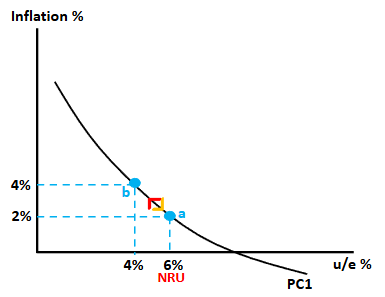
Expectations and the money illusion

The original Phillips Curve assumed static inflation expectations (e.g. 2%).
If the government boosts AD to cut unemployment below the natural rate (e.g. 6% → 4%), firms raise money wages.
Workers suffer money illusion, mistaking higher money wages for higher real wages, so labour supply rises temporarily.
As wage rises feed into higher inflation (e.g. 4%), real wages are unchanged → workers leave employment → unemployment returns to the natural rate.
Inflation then falls back as AD weakens.

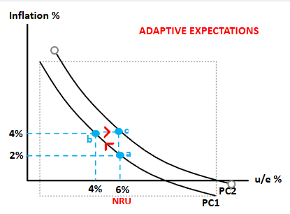
Adaptive expectations and the Phillips curve

• Government boosts AD to cut unemployment below the natural rate (e.g. 6% → 4%).

• Workers initially experience money illusion, increasing labour supply → economy moves up the Phillips Curve.

• Higher wages cause higher actual inflation; workers realize real wages haven’t risen → unemployment returns to natural rate.

• After repeated experience, workers expect higher inflation (e.g. 4%), so the Phillips Curve shifts upward, and attempts to reduce unemployment below the natural rate only raise inflation.

Inflationary consequences of targeting lower unemployment

• To keep unemployment at 4%, money wages must rise faster than inflation.

• If inflation is expected at 4%, wages rise 6% → perceived +2% real wage → move up the Phillips Curve (point D).

• As expectations rise (to 6%, then 8%), wages must increase even more (8%, then 10%) to maintain the same real wage gain.

• Outcome: ever-higher inflation with no long-run reduction in unemployment.

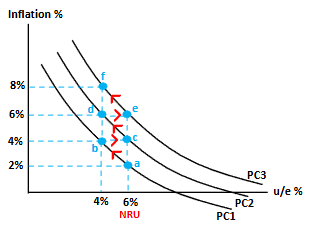
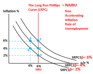
Expectations-Augmented and long run Phillips curve

• Expectations-augmented Phillips Curves: “stacked” curves, each based on a given expected inflation rate (ṗ).

• NRU is vertical and intersects each curve where expected inflation = actual inflation.

• At this point, real wages are correct → stable employment.

• This vertical line is the Long-Run Phillips Curve (LRPC).

• The individual stacked curves are Short-Run Phillips Curves (SRPCs).

• Keeping unemployment below the NRU requires continually boosting AD → accelerating inflation.

• LRPC is also called NAIRU: unemployment rate with no accelerating inflation.

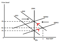
AD/AS explanations of the Phillips curve

• Yf/e = full employment (natural rate): all willing/able workers employed at the going real wage.

• Govt boosts AD → shifts right (AD₂).

• Economy moves up SRAS₁ → output rises above Yf/e to Y, prices rise to P₂.

• Output exceeds capacity due to overtime & temporary workers, raising costs.

• Higher costs shift SRAS left to SRAS₂.

• Economy returns to Yf/e but at a higher price level (P₃).

• Conclusion: boosting AD causes temporary GDP/employment gains, but permanent inflation.

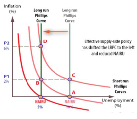
Does the Phillips curve trade-off still exist?

• 1993–2008: UK unemployment fell to record lows without rising inflation, contradicting the original Phillips Curve.

• Explanation: effective supply-side policies (SSPs).

• SSPs increase productive capacity → economy can grow without inflation.

• Result: Long-Run Phillips Curve shifts left (equivalent to LRAS shifting right).

• Lower inflationary expectations → movement to a lower Short-Run Phillips Curve (SRPC).

What is the Keynesian view of the the lower NRU due to SSPs?

Policies that have dealt with structural unemployment have improved skills in the economy enabling more people to take up work e.g. more spending on education etc

What is the classical view of the lower NRU due to SSPs?

Policies that have dealt with voluntary unemployment have incentivised work, meaning more people to choose work over life on benefits e.g. cutting benefits etc.

Insights from LRPC analysis

• LRPC shifts caused by structural change & supply-side policies.

• SRPC shifts caused by changes in inflationary expectations.

• 1970s stagflation:

  • Rising NAIRU (LRPC → right) from industrial decline.

  • Expansionary policy raised expectations → SRPC shifted up.

• Short run Phillips Curve still holds: higher expected inflation → higher SRPC.

• Inflation targeting keeps expectations low → lower SRPC.

• 1990s disinflation:

  • NAIRU fell (LRPC → left) due to SSPs.

  • BoE independence reduced expectations → SRPC shifted down.