FINS3625 Applied Corporate Finance

First principles

Goals of a business

• Obviously maximize the value of the firm

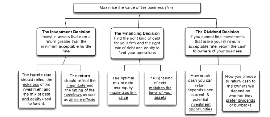
Maximizing value of the firm

• Done through by the:

  • Investment Decision

    • Investing in assets that earn a return greater than the minimum acceptable hurdle rate

  • Financing Decision

    • Finding the right kind of debt for the firm and the right capital structure (mix of debt and equity) to fund operations

  • Dividend Decision

    • If unable to find investments that succeed the minimum acceptable rate, return the cash to owners (shareholders) through dividends

Investment Decision

• Made up of:

  • the hurdle rate

    • reflects the riskiness of the investment and the mix of debt and equity used to fund it

  • the return

    • reflects the magnitude and timing of cash flows as well as all side effects

Financing Decision

• Made up of:

  • the optimal mix of debt and equity maximizing firm value

  • the right kind of debt matches tenor of assets

Dividend Decision

• Made up of:

  • Amount of cash that can be returned depends on current and potential investment opportunities

  • Method of returning cash depends whether they prefer dividends or buybacks

Hurdle Rate as a benchmark

• Since financial resources are finite, there is a hurdle that projects have to cross before being deemed viable, hurdle rates should change for riskier projects

• Simple representation is: Hurdle Rate = Risk-Free Rate + Risk Premium

• The two basic questions that every risk and return model tries to answer when determining this will be:

  • How to measure risk

  • How to translate the risk measure into a risk premium value

Features of a good risk model

• measure of risk should be applicable to all asset types

• should delineate what types of risk are rewarded and whcih are not

• should come with standardised risk measures and should be able to draw conclusions whether an asset is above or below average

• it should translate the measure of risk into a rate of return that the investor should demand as compensation for bearing the risk

• should work well not only at explaining past returns but also in predicting future expected returns

Capital Asset Pricing Model (CAPM)

• Uses variance of actual returns around an expected return as a measure of risk

• Specifies that a portion of variance can be diversified away, and that will be the only non-diversified portion that is rewarded

• Measures the non-diversifiable risk with beta which is standardised around one

• Translate beta into expected return

  • Expected return = Risk free rate + Beta * Risk Premium

• Works as well as the best next alternative in most cases

Importance of Diversification

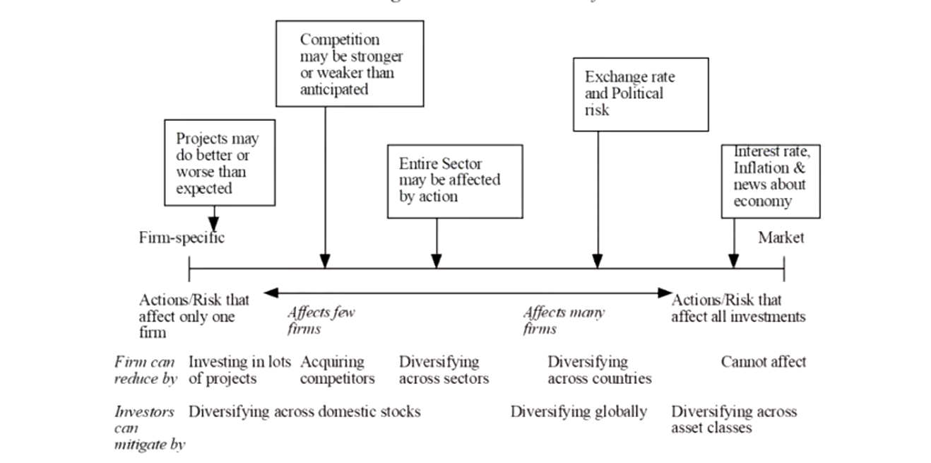
Why diversification reduces / eliminates firm specific risks

• Firm specific risk can be reduced / eliminated by increasing the number of investments in the portfolio, market wide risk cannot, as they can be justified on either economic or statistical grounds

• On economic grounds, diversifying and holding a larger portfolio eliminates firm specific risk for two reasons:

  • Each investment is a much smaller percentage of the portfolio, muting the effect (positive/negative) on the overall portfolio

  • Firm specific actions can be either positive or negative, in am large portfolio, the effects will average out to be zero as for every firm doing bad there is one doing well in the portfolio

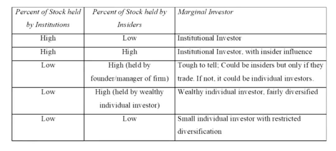
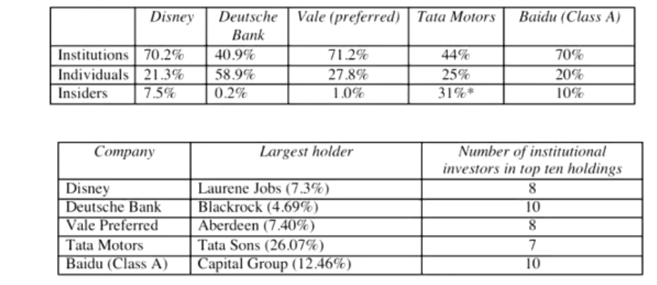
The role of the marginal investor

• Entity / individual in a firm who is most likely to be the buyer or seller on the next trade and to influence the stock price

• Generally speaking, the marginal investor in a stock has to own a lot of stock and also trades that stock on a regular basis

• Since trading is required, the largest investor may not always be the largest investor

• In all risk and return models, it is assumed that the marginal investor is well diversified

• In most public companies they are institutional holders (Vanguard, State Street, Blackrock)

Identifying the marginal investor and real life examples

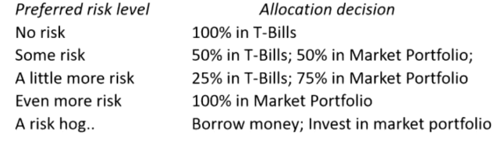
The market portfolio

• Assuming diversification costs nothing (in terms of transaction costs), and that all assets can be traded, the limit of diversification is to hold a portfolio of every single asset in the economy (in proportion to market value). This portfolio is called the market portfolio

• Individual investors will adjust for risk by adjusting their allocations to this market portfolio and a riskless asset

Risk of an individual asset

• Risk of any asset is the risk that it adds to the market portfolio statistically, this risk can be measured by how much an asset moves with the market (called the covariance)

• Beta is the standardised measure of this covariance, obtained by dividing the covariance of any asset with the market by the variance of the market. This is the measure of the non diversifiable risk for any asset which can be measured by the covariance of its returns with returns on a market index which is defined to be the asset’s beta

• The required return on investment will be a linear function of its beta:

  • Expected Return = Risk free rate + Beta * (Expected return on the market portfolio - Risk free rate)

Limitations of the CAPM

• Model makes unrealistic assumptions

• Parameters of the model cannot be estimated precisely

  • The market index used can be wrong

  • The firm may have changed during the estimation period

• The model does not work well

  • If the model is right there should be:

    • A linear relationship between returns and betas

    • The only variable that could explain returns is betas

  • The reality is that

    • The relationship between betas and returns is weak

    • Other variables seem to explain differences in returns better (this could be size, price/book value)

Alternatives to CAPM

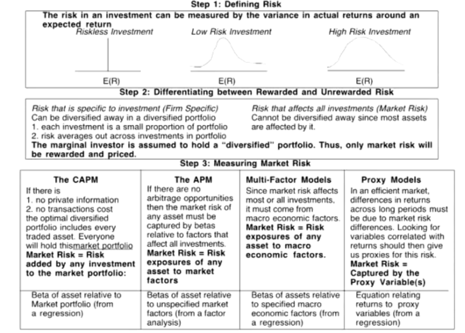
Why CAPM remains the most prevalent

• Alternative models do a much better job at explaining past returns but their effectiveness drops off when it comes to estimating expected future returns as the models tend to shift and change

• Alternative models are more complicated and require more information to work compared to CAPM

• For most companies the expected return you get with the alternative models is not different enough to be worth the extra trouble of estimating 4 additional betas

Inputs required for the CAPM

• CAPM yields the following expected return

  • Expected return = Risk free rate + Beta * (Expected Return on the market portfolio - risk free rate)

• To use the model we need these inputs:

  • The current risk free rate

  • The expected market risk premium, the premium expected for investing in risky assets

  • The beta being analysed

Risk free rate and time horizon

• On a risk free asset the actual return is equal to the expected return, therefore there is no variance around the expected return

• For an investment to be risk free (actual return = expected return), two conditions must be met -

  • No default risk which implies it has ton be a government security, however not all governments can be viewed as default free

  • No uncertainty about reinvestment rates (which implies that it is a ZCB with the same maturity as the cash flow being analysed)

Risk free rate in practice

• Risk free rate is the rate on a zero coupon default free bond that matches the time horizon of the cash flow being analysed

• This translates into using different risk free rates for each cash flow, 1 Year ZCB for Year 1, Year 2 ZCB for Year 2 and so on

• Practically speaking if there is uncertainty about expected cash flows, the present value effect of using time carrying risk free rates is small enough that it may not be worth it

• In corporate finance, most scenarios are long term therefore using a long term default free rate as the risk free rate makes sense (typically a 10 year gov bond)

Denomination of Risk Free Rates

• The risk free rate used in the analysis should be in the same currency that your cashflows are estimated in, Euro Cashflows = Euro Risk Free rate, USD Cashflows USD Risk Free rate

• The conventional practice is to use the government bond rate with the government being the one in control of issuing the currency

  • For the Euro which is the currency of a number of countries, typically the risk free rate would be associated with the most stable country (typically Germany or alternatively if no government is not default free the ECB)

• If the government is default free using a long term government rate (even on a coupon bond) as the risk free rate will yield a close approximation of true value (ex: 10 year treasury bond)

What to do if theres no default free entity

• Adjust the local government borrowing rate for default risk to get a riskless currency rate

  • this can be done by subtracting the bond rate with the default spread for a bond of the country’s credit rating

• Analyse in an alternate currency where the risk free rate is easily obtainable, this can be the US treasury bond rate

• Analyse in real terms in which case the risk free rate has to be a real risk free rate, the inflation indexed treasury rate is one such example of a real riskfree rate

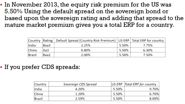
Paths to estimating sovereign default spreads

• Sovereign Dollar or Euro dominated bonds

  • difference between the interest rate on a sovereign US$ bond issued by the country and the US treasury bond rate can be used as the default spread

• Credit Default Swap (CDS) spreads

  • Obtain the default spreads for sovereigns in the CDS market

• Average spread

  • The country’s sovereign rating can be used to estimate the default spread based on the default spread for the rating

Equity Risk Premium

• Premium that investors demand for investing in an average risk equity relative to the risk free rate, price of risk in equity markets rising with fear

• Generally the premium should be:

  • Greater than zero

  • Increase with the risk aversion of investors in the market

  • Increase with the riskiness of the “average” risk investment

• If so it also follows that equity risk premiums should change over time, as economic circumstances change and investor composition also change

Estimating risk premiums

• Survey premiums

  • Survey investors on their desired risk premiums and use average premium from these surveys

• Historical premiums

  • Assume that the actual premium delivered over long time periods is equal to the expected premium delivered over long time periods is equal to expected premium

• Implied premiums

  • estimate a forward looking premium based upon today’s asset prices

Survey Approach

• Surveying all investors in a market is impractical

• However surveying a few individuals is possible and use the results to provide an estimation

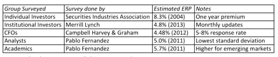
However:

• There are no constraints on reasonability (the survey could produce negative risk premiums or risk premiums of 50%)

• The survey results are more reflective of the past than the future

• Tend to be short term as the longest surveys do not go beyond one year

Historical ERP Approach

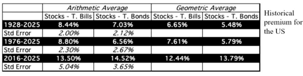
A historical risk premium has to be:

• Long term (because of the standard error)

• Consistent with choice of risk free rate

• A “compounded” average

No matter which estimate used recognise that it is backward looking, noisy and may reflect selection bias

Limitations:

• Data quality for markets outside the US is available for much shorter time periods, the problem is even larger in emeging markets

• Historical premiums that emerge from this data reflects this data problem and there is much greater error associated with the estimates of the premiums

Implied ERP Approach

• Through identifying the prices that investors are willing to pay for stocks it is possible to find an expected return and hence the implied equity risk premium

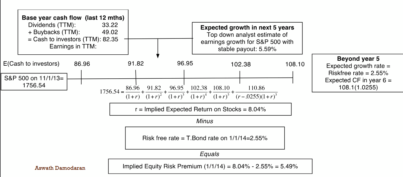
• Use current market level (S&P 500) as price today

• Estimate cash flows to equity investors:

  • Dividends + Share buybacks

  • Base cash flow ≈ 82.35

• Forecast cash flow growth (next 5 years):

  • Growth rate ≈ 5.59%

  • Generate yearly cash flows (Yr 1 → Yr 5 increasing)

• Estimate terminal value (after year 5):

  • Assume growth = risk-free rate (2.55%)

  • Use Gordon Growth formula:

    • TV = Final cash flow × (1 + g) / (r − g)

• Discount all cash flows to present:

  • Price = PV of (Years 1–5 cash flows + Terminal Value)

• Solve for r (implied expected return):

  • r ≈ 8.04%

• Compute Equity Risk Premium (ERP):

  • ERP = Expected return − Risk-free rate

  • ERP = 8.04% − 2.55% = 5.49%

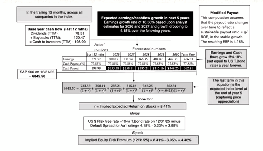
Updated implied ERP (2025 Example)

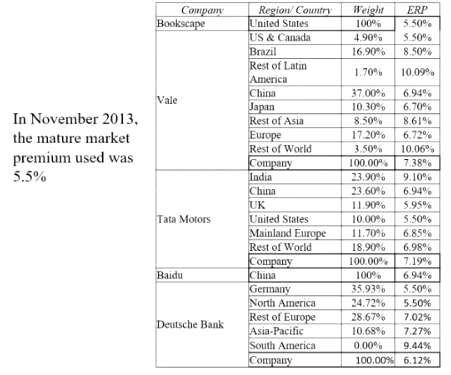
ERP for other markets

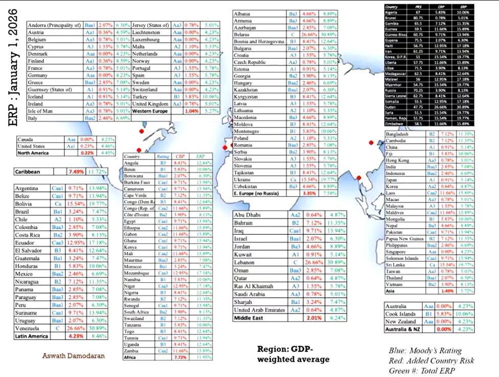
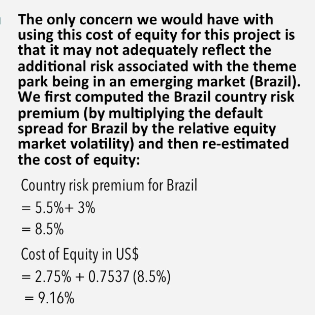
Equity risk premium for emerging markets

• Mature and Emerging markets will have different ERPs due to emerging markets being riskier therefore to calcuilate ERP for emerging markets:

  • Use melded default spread approach (default spread set by ratings agency scaled up to reflect the risk of holding equity) shown here:

  • Emerging Market ERP: Mature Market ERP + Country Deficit Spread * (Std of equity / Std of country bond)

Example of using bond default spreads for ERP

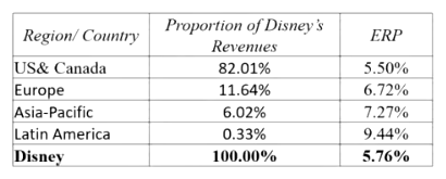
Estimating an ERP for a company that operates muiltinationally

• The conventional practice is to only estimate an ERP based upon where the company is incorporated, thus a US based company with operations overseas would be computed based on US ERP and a chinese company with operations mainly in the US would still use a Chinese ERP.

• However the more sensible practice (Damodaran) is to estimate ERP based upon where the company operates example below:

Estimating Beta

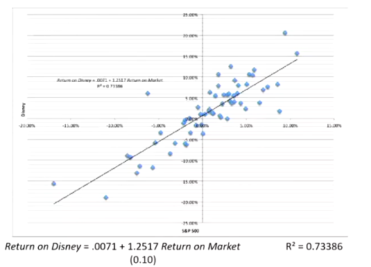
• The standard procedure for estimating betas is to regress stock return (Rj) against market returns (Rm)

  • Rj = a + b Rm

    • a is the intercept

    • b is the slope of the regression (beta)

• The slope of the regression corresponds to the beta of the stock and measures the riskiness of the stock, note that regression parameters are always estimated with error

• The R-squared (R²) of the regression provides an estimate of the proportion of the risk (variance) of a firm that can be attriuted to market risk. The balance can be attributed to firm-specific risk.

• note that technically this is not correct form as we should be using excess returns and the CAPM formula to calculate beta:

• Rj​ − Rf​ = α + β (Rm ​− Rf​)

• Due to the availability of more data, it is increasingly more common to use daily or weekly data, this frequency allows us to eliminate the subtraction of the risk free rate as it is negligible. Higher frequencies (monthly and up) will require this subtraction however.

Estimating Performance

• The intercept of a regression provides a simple measure of performnance during the period of regression relative to the CAPM

  • Rj = Rf + b (Rm - Rf)

  • = Rf (1-b) + b Rm …. CAPM

  • Rj = a + b Rm …. Regression Equation

• if a > Rf (1-b) …. the stock did better than expected during the regression period (*unsure check w PASS* High market exposure → expected return is heavily driven by market risk.)

• if a < Rf (1-b) …. the stock did worse than expected during the regression period (Lower market exposure → more of return comes from risk-free component.

• if a = Rf (1-b) …. the stock did as well during the regression period (stock moves one for one with the market)

• The difference between the intercept and Rf (1-b) is Jensen’s alpha. If it it is posiotive the stock performed better than expected durting the period of regression

setting up for an estimation

• Decide on an estimation period

  • Services use period ranging from 2-5 years for the regression

  • Longer estimation periods provide more data but firms change

  • Shorter periods are easily affected by firm specific events that might occur during the period

• Decide on a return interval

  • Shorter intervals yield more observations but suffer from more noise

  • Noise is created by stocks not trading and biases all betas towards one

• Estimate returns (including dividends) on stock

  • Return (HPR) = (PriceEnd - PriceBeginning + DividendsPeriod) / PriceBeginning

  • Included dividends only in ex-dividend month

• Choose a market index and estimate returns (inclusive of dividends) on the index for each interval for the period

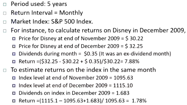
• Typically we use weekly or daily frequencies nowadays for more reliability

• Industry betas can also be used for estimating a company’s beta as this method is more stable, however not all companies can match the industry

Finding and Analysing performance

• Intercept = 0.712%

  • This is essentially the monthly return of Disney, and has to be compared to a monthly risk free rate (to measure how good our return is)

  • Between the periods (assuming a US Company)

    • Average annual T bill rate = assumed to be say 0.5%

    • Monthly risk free rate will be: 0.5/12 = 0.042%

    • Risk free rate (1-Beta) = 0.042% (1 - 1.252) = -0.105%

• In order to find just how well disney performed:

  • Intercept - Risk free rate (1-Beta)

  • 0.712% - (-0.105%)

  • Jensen’s Alpha is then = 0.723%

• This means the company did 0.723% better than expected per month between the periods

• Ensure to annualise the excess return giving: annual excess return = (1 + Alpha)^12 - 1

• Or: annual excess return (1 + 0.0723)^12 - 1 = 9.02%

Breaking down Risk

• Say that R Squared = 73%

• This implies that

  • 73% of the risk of the company comes from market sources

  • 27% comes from firm specific sources

• firm specific risk is diversifiable and will not be rewarded

Inputs to the expected return calculation

• Company Beta = 1.25

• Risk free rate = (US ten year TBond rate at whatever period)

• Risk premium = 5.76% (based on company’s operating exposure in different countries,etc)

• Expected return = Risk free rate + Beta (risk premium)

enterprise value

• calculated as market value of equity + debt - cash

• Used for EV/Sales calculations amongst peer group

  • This can then be used for calculating the value of the business unit

firm value

• calculated as market value of equity + debt

What does the expected return mean to investors

• It is the expected return that an investor can expect to make in the long term on the company if the stock is correctly priced and CAPM remains the right model for risk

• it is the return that an investor needs to make on the company in the long term to break even on the investment in the stock

• Both

What does the expected return mean to the company

• Need to make at least 9.95% as a return for their equity investors to break even.

• This is the hurdle rate for projects, when the investment is analyzed from an equity standpoint

• Therefore the cost of equity is 9.95%

top down vs bottom up beta

• top down beta comes from the regression beta (levered beta)

• bottom up beta is estimated by:

  • Finding what industry the business operates in (this can be more than one)

  • Find the unlevered firms of companies that are operating in the same industries

  • Take a weighting (by sales or operating income) average of these betas

  • lever up using the firms D/E

Why use bottom up beta

• the betas can reflect the current and even expected future mix of businesses the firm is in rather than the historical mix

• The standard error of the beta estimate will be much lower

• make judgment on different businesses within the company as we can estimate cost of equity by business

Fundamentals that drive beta

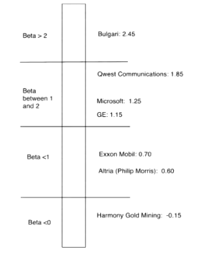
• Beta > 2: indicates that the company is very cyclical and theres a big risk associated with the broad market (say if the economy tanks)

• Beta between 1 and 2: leaning more towards the higher side might indicate that the company has high fixed costs that make it risky, leaning towards 1 means that the company is well diversified enough in the sense that it has cash accumulated and is stable

• Beta < 1: companies that are not moving with the market as much, an example would be oil, defence companies that do well when there is instability. Another example is cigarette producers which move slow and rely on addiction

• Beta < 0: companies that move in the opposite direction of the market an example is gold mining companies, typically used as a hedge / insurance

Product / Service type as a determinant of beta

• Betas measure a company’s exposure to macroeconomic risks. Consequently, you would expect the beta to be a function of the sensitivity of the demand for its products and services to macroeconomic factors

  • To the extent that cyclical companies are more likely to move with the macroeconomy, they are likely to have higher betas

  • Firms which sell more discretionary products will have higher betas than firms that sell less discretionary product

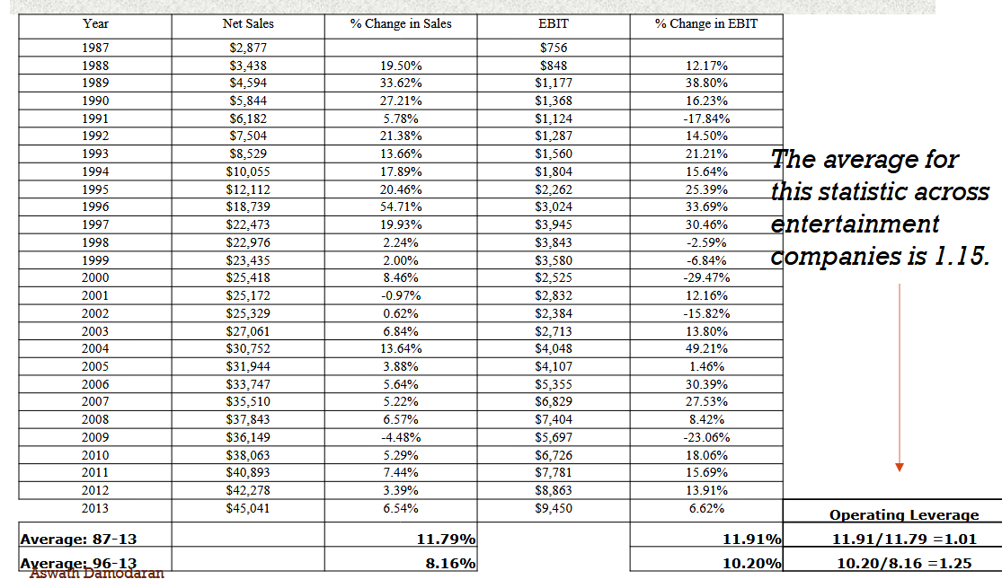
Operating leverage effects

• Operating leverage refers to the proportion of the total costs of the firm that are fixed.

• When a company has higher fixed costs, small changes in revenues will translate into larger changes in earnings, and by extension, into more variable earnings

  • Other things remaining equal, sectors with higher operating leverage should have higher betas than sectors with less operating leverage.

  • Within sectors, companies with more flexible cost structures (where costs adjust more quickly to revenues) should have lower betas than companies with more rigid cost structures.

Measures of operating leverage

• Fixed costs measure: Fixed costs / Variable costs

  • Measures the relationship between fixed and variable costs. The higher the proportion the higher the operating leverage

  • The problem with this measure is that companies do not break costs down into fixed and variable costs

• EBIT Variability measure: % Change in EBIT / % Change in Revenues

  • Measures how quickly the earnings before interest and taxes changes as revenue changes, the hgiher the number the greater the operating leverage

  • There is noise in this number on a YtY basis

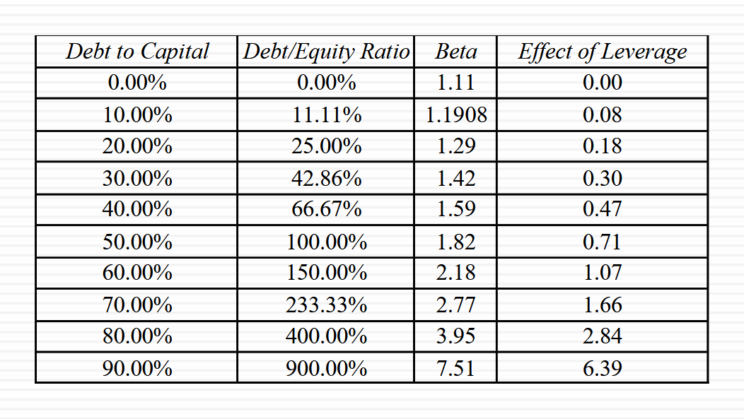
Financial Leverage as a determinant of beta

• As firms borrow they create fixed costs (interest payments) that make their earnigns to equity investors more volatile, this increased earnings volatility increases the equity beta

• beta of equity alone can be written as a function of the unlevered beta and the debt-equity ratio

• Regression betas are levered as it based on stock prices which reflect leverage

Betas are weighted averages

• Betas of a portfolio is always the market value7 weighted average of the betas of the individual investments in that portfolio

• Thus,

  • the beta of a mutual fund is the weighted average of the betas of the stock and other investments in that portfolio

  • the beta of a firm after a merger is in the market value weighted average of the betas of the companies involved in the merger

Pure play beta calculation

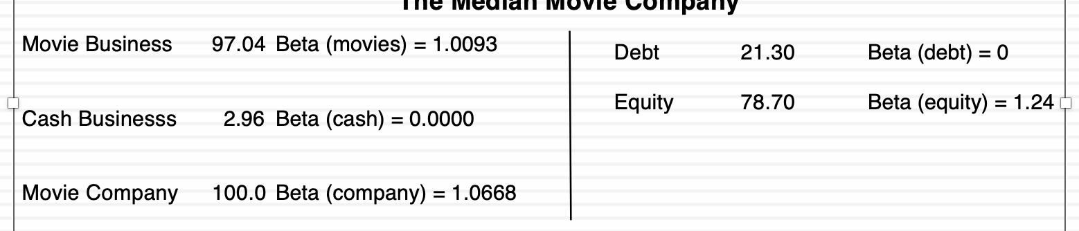
• start with the median regression beta (equity beta) in this case being 1.24

• unlever the beta using the median D/E ratio of 27.06%

  • Gross D/E: 21.30/78.70 = 27.06%

  • Unlevered beta: 1.24 / (1-(1-T)(0.2706))

    • T assumed to be 40%

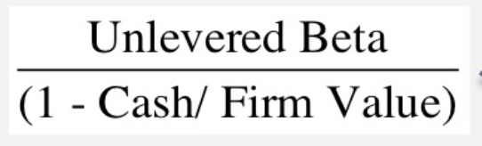
  • Take out the cash effect using the median cash / value of the business

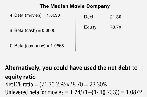
    • (0.2960)(0) + (1-0.2960)(Beta of movie business) = 1.0668

    • Revenue x Beta of cash + Revenue x Beta of movie = beta of movie company

    • Beta of movie business: 1.0668 / (1-0.2960) = 1.0993

  

  • Using net debt equity ratio

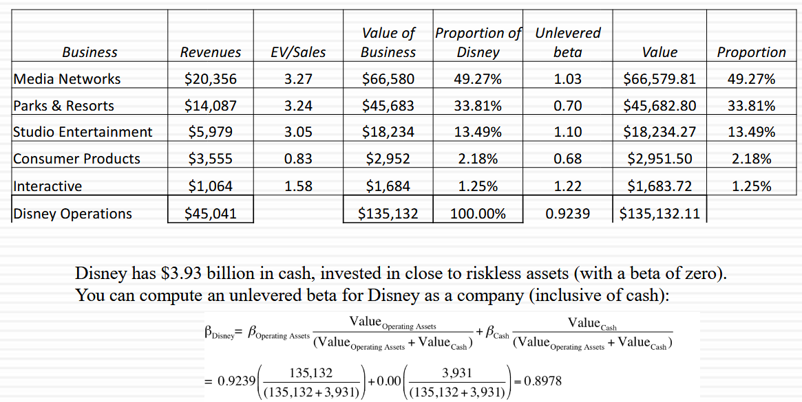
Finding the final unlevered beta for the whole company

• It is possible to compute an unlevered beta for the company once the unlevered beta for all its operations are calculated

• Example:

Levered beta for company and divisions from unlevered beta

• Since debt sits at the corporate level, Damodaran allocates it proportionally by identifiable assets — the logic being that assets are what the debt is financing.

  • Calculate the Division D/E ratios, example:

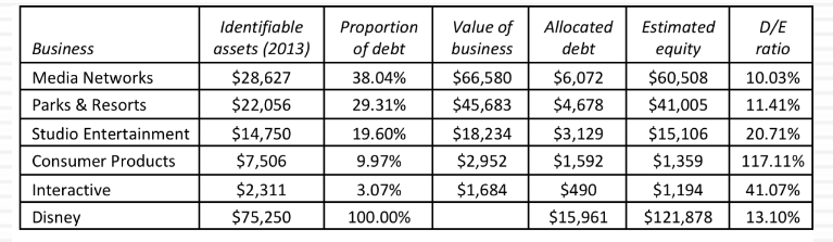
• Allocated Debt = (Division Assets / Total Assets) × Total Debt

  • Estimated Equity = Value of Business − Allocated Debt

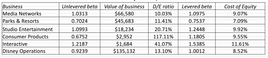
• Each division gets an unlevered beta (from comparable industry firms), then re-levered using its own D/E ratio:

  • Levered Beta = Unlevered Beta × (1 + (1 - tax rate) × D/E)

• Finally Using CAPM:

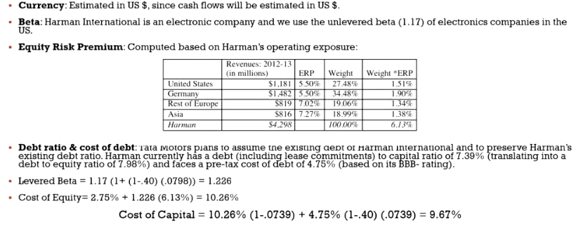
  • Cost of Equity = Risk-free Rate + Beta × ERP = 2.75% + Beta × 5.76%

Cost of equity calculation in terms of other currencies

• Converting a discount rate in one currency to another, all that is needed are expected inflation rates in the two currencies ex:

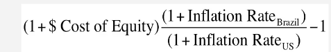
• For the US generally it is the difference between the TIPS rate and the 10 Year T-Bond rate

• Generally is better this way as so many of the risk premiums (ERP, CDS) all come from dollar based markets

Estimating betas for non traded assets

• the conventional approaches of estimating beta from regressions do not work for assets that are not traded, there are non stock prices or historical returns that can be used to compute regression betas

• Two ways that betas can be estimated for non traded assets

  • Using comparable firms

  • Using accounting earnings

Estimating a private company’s levered beta and cost of equity

• Debt to equity ratios are market debt equity ratios and often the only debt equity ratio available is a book value debt equity ratio, it can be assumed that the company is close to the industry median market debt to equity ratio

• Using a marginal tax rate, it is possible to get the levered beta

• Using a risk free rate it is possible to find the ERP

• Beta measures the risk added to a diversified portfolio, the owners of small companies are not diversified and therefore will result in an underestimation/overestimation for cost of equity

• Adjust the beta to reflect total risk

  • Total Beta = Market Beta / Correlation of the sector with the market

• total cost of equity will be the risk-free rate plus this total beta

• DAMADORAN SESSION 11

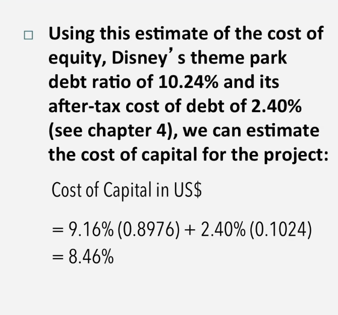
From cost of equity to cost of capital

• Cost of capital is a composite cost to the firm of raising financing to fund its projects

• In addition to equity, firms can raise capital from debt

• To get a cost of capital:

  • Estimate a cost of debt

  • Estimates weights for debt and equity

What is debt?

• General rule: Debt generally has the following characteristics:

  • Commitment to make fixed payments in the future

  • The fixed payments are tax deductible

  • Failure to make the payments can lead to either default or loss of control of the firm to the party whom payments are due

• As a consequence debt should include

  • any interest bearing liability, whether short or long term

  • any lease obligation whether operating or capital

Estimating the cost of debt

• If the firm has bonds outstanding and the bonds are traded, the YTM on a long term, straight (no special features) bonds can be used as the interest rate

• If the firm is rated, use the rating and a typical default spread on bonds with that rating to estimate the cost of debt

• If the firm is not rated

  • and it has recently borrowed long term from a bank, use the interest rate on the borrowing or

  • estimate a synthetic rating for the company, and use the synthetic rating to arrive at a default spread and a cost of debt

• cost of debt has to be estimated in the same currency as the cost of equity and the cash flows in the valuation.

Outsourcing the measurement of default risk

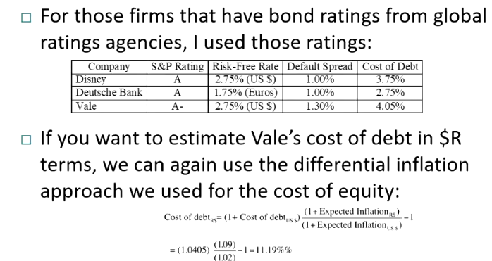
Estimating synthetic ratings

• Rating for a firm can be estimated using the financial charactheristics of then firm, in its simplest form, this is the interest coverage ratio.

• Interest coverage ratio = EBIT / Interest Expense

• Example for non financial service companies

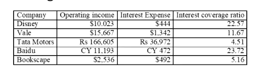
• Indicates how many multiples of income is going to cover your interest for Bookscape, every $5 it earns $1 goes to interest expense

Interest Coverage Ratios, Ratings and Default Spreads

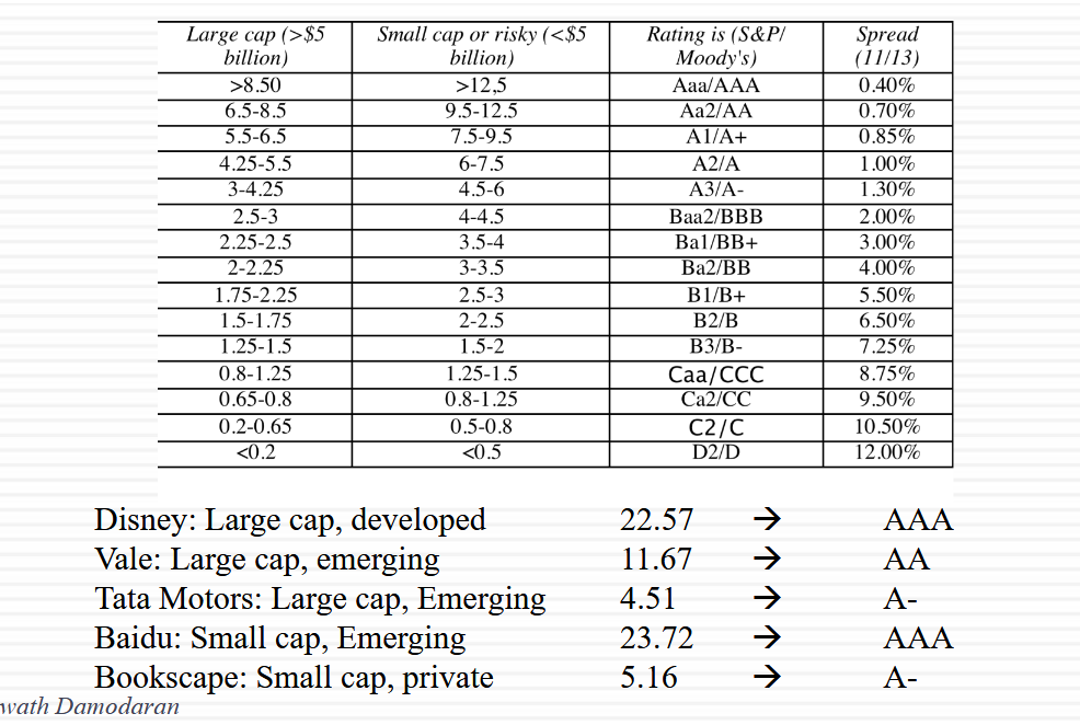
• Calculate the ICR for the company

• Determine company size — Large cap (>$5B) or Small cap/risky (<$5B)

• Find the matching ICR range in the corresponding column

• Read off the rating from the S&P/Moody's column

• possible emerging market adjustment (typically 1 notch down) reflecting volatility, currency / political risk and sovereign / country risk of operating in an emerging market

Synthetic vs Actual Ratings

• A firm’s synthetic rating may differ from its actual rating as:

  • Synthetic ratings reflect only the ICR whereas actual ratings incorporate all other ratios and additional qualitative factors

  • Synthetic ratings do not allow for sector wide biases in ratings

  • Synthetic ratings was based on the year’s operating income whereas actual rating reflects normalised earnings

• Another key factor that can differ synthetic and actual ratings is the presence of country risk, emerging market companies get rated lower

• Banks are generally not advised to measure using synthetic ratings as defining interest expenses for a bank may be difficult

Estimating cost of debt

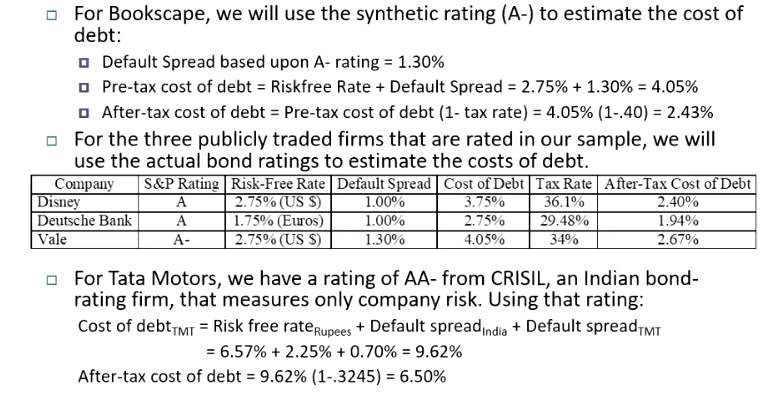
• Debt is tax deductible hence the adjustment for after-tax debt leading to a lower true cost for the firm when using debt financing

• For Tata cost of debt has three components:

  • 6.57% — Indian rupee risk-free rate (already embeds Indian inflation)

  • 2.25% — India's sovereign default spread (country risk)

  • 0.70% — Tata Motors' additional company-specific spread (AA- rating)

• Essentially:

  • Private firm → synthetic rating

  • Public firm, developed market → actual rating + matching risk-free rate

  • Public firm, emerging market → must add a country risk layer on top

Preferred stock

• Shares some of its characteristics with debt:

  • Preferred dividend is pre-specified at the time of issue

  • Paid out before common dividend

• However they share some characteristics of equity;

  • not being tax deductible

• If preferred stock is viewed as perpetual then the cost of preferred stock is:

Preferred dividend per share / market price per preferred share

Convertible debt

• part debt (bond part) and part equity (convertible part)

• best to break up the component parts and eliminate it from the mix altogether

Weights for cost of capital calculation

• Weights used in the cost of capital calculation should be market values, this is because cost is a forward looking measure based on debt, equity values today in regard to how its effectively raising the cash

• Using book value will result in:

  • a lower cost of capital than using market value weights

  • while it may seem consistent to use book values for both accounting return and cost of capital calculations, it does not make economic sense

  • book value is not as volatile (stays the same regardless of financial health)

book value of debt to market value for WACC

• Debt isn’t always traded therefore there may not be a market value for debt. Therefore we treat all debt as a single coupon bond and calculate its present value

• From financial statements:

  • Total book value of debt acts as the face value

  • Annual interest expense acts as the coupon

  • Pre-tax cost of debt acst as the discount rate

  • Weighted average maturity

    • sum of (weight x time)

    • allows us to represent all of Disney’s debt as one equivalent bond

Example:

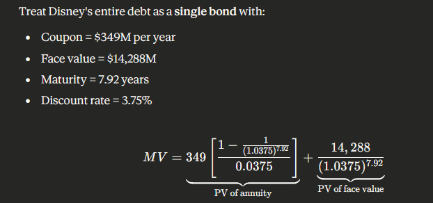
• PV of the annuity captures the interest payments

• PV of face value captures the repayment of the principal

• The market value being lower indicates that investors would pay less than face value for the debt as the coupon payments are lower than the current market rate (349M / 14288M)

  • if coupon payments are higher the debt will trade at a premium as investors will be willing to pay more than face value

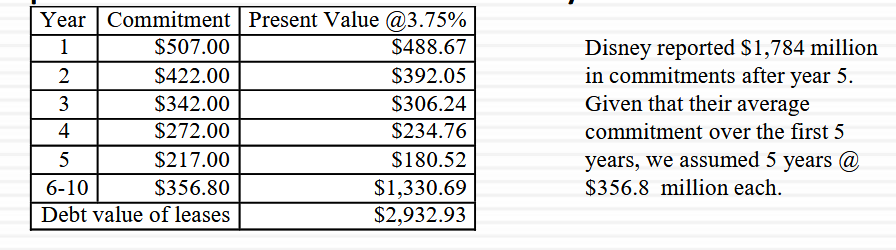
Operating leases

• Fixed commitment of lease payments over a number of years, hence are thought of as debt and are tax deductible

• debt value of operating leases is the present value of the lease payments at a rate that reflects their risk usually the pre tax cost of debt

• sometimes the entire lease payments aren’t disclosed therefore use an average of the years that are disclosed for the period that we need (say 10 years)

• Total debt is then

  • Interest bearing debt + lease debt

  • Provides a complete picture of Disney’s true financial obligations for use in WACC.

Choosing a hurdle rate

• Cost of equity or cost of capital can be used as a hurdle rate, depending upon whether the returns measured are to equity investors or to all claimholders on the firm’s capital

• if returns measured are to equity investors use cost of equity

• if returns measured are to all claimholders use cost of capital

Measures of return: earnings vs cash flows

• Principles governing accounting earnings measurement

  • Accrual accounting: show revenues when products and services are sold or provided not when they are paid for. Show expenses associated with these revenues rather than cash expenses (Sell at 31 Dec but not paid will still show up in the statements for that year)

  • Operating vs CapEx: expenses associated with creating revenues on the current period should be treated as operating expenses (rent). Expenses that create benefits over several periods are written off over multiple periods (as depreciation or amortisation)

• To get from accounting earnings to cash flows have to:

  • add back non-cash expenses (depreciation, share repurchases), lower earnings but not cash

  • subtract out cash outflows which are not expected (such as CapEx)

  • make accrual revenues and expenses into cash revenues and expenses (by considering changes in working capital, aka accounts receivable, inventory, etc)

Measuring returns right

• use cash flows instead of earnings, as you cannot spend earnings

• use “incremental cash flows” relating to the investment decision i.e cashflows that occur as a consequence of the decision, rather than total cash flows (sunk costs not included)

• Use “time weighted” returns i.e value cash flows that occur earlier more than cash flows that occur later

  • The return mantra is “time-weighted”, incremental cash flow return”

What is an investment

• An investment or project can range from being small to big, money making to cost saving:

  • Major strategic decisions

  • Acquistions of other firms are projects as well

  • Decisions on new ventures

  • Decisions that may change the way existing ventures and projects are ruin

  • Decisions on how best to deliver a service that is necessary for the business to run smoothly

• Every choice a firm makes can be an investment

Examples of projects

• At Disney,

  • Rio Disney: Consider whether Disney should invest in its first theme parks in South America. These parks will require us to consider the effects of country risk and currency issues in project analysis

  • A New Show for Disney Plus: An exercise where estimating the benefits is difficult to do, since it is in the form of keeping existing subscribers or adding new ones

• New iron ore mine for Vale: This is an iron ore mine that Vale is considering in Western Labrador, Canada.

• An Online Store for Bookscape: While it is an extension of their basis business, it will require different investments (and potentially expose them to different types of risk)

• Acquisition of Harman by Tata Motors: cross-border bid by Tata for Harman International, a publicly traded US firm that manufactures high-end audio equipment, with

  the intent of upgrading the audio upgrades on Tata Motors’ automobiles. The investment

  will allow us to examine currency and risk issues in such a transaction.

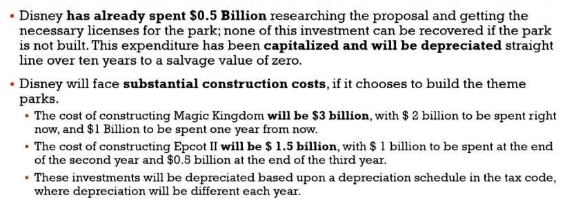
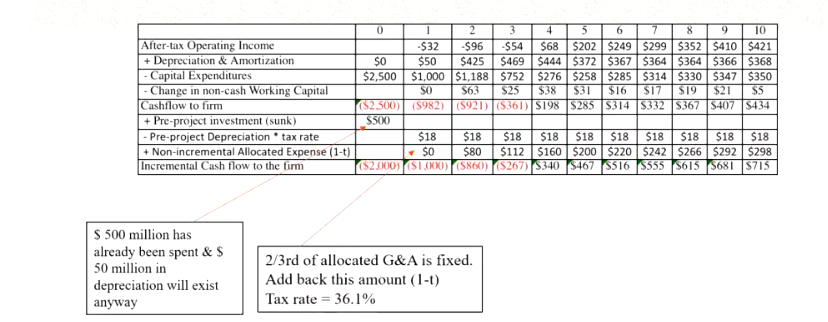
Disney new theme park project

• Costs incurred that are already sunk

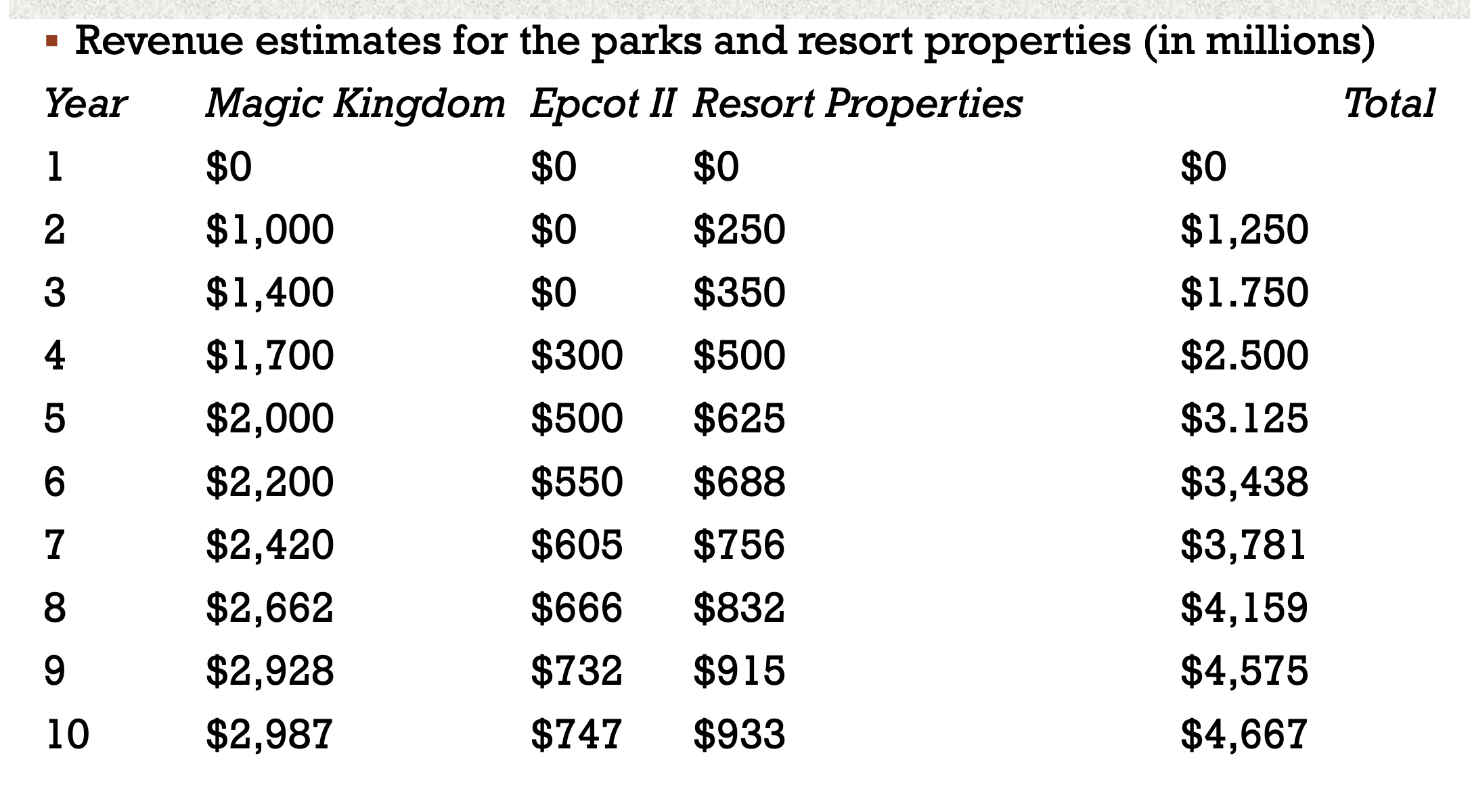
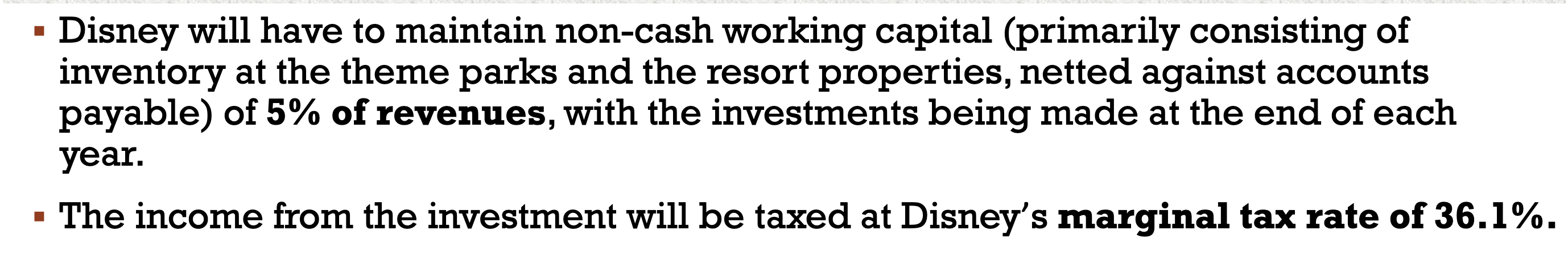
• Revenue assumptions are based on Damadoran’s calculations

  • no revenues in Y1 due to construction (losses can be used to reduce the tax burden elsewhere in the firm until profits come)

  • used 25% of themepark revenues for hotel revenues

  • used how euro disney built up over time and those revenues

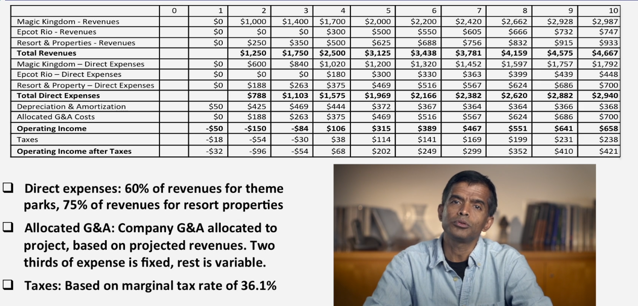
• ^^ ensure to also subtract the depreciation and armotisation due to them being accounting

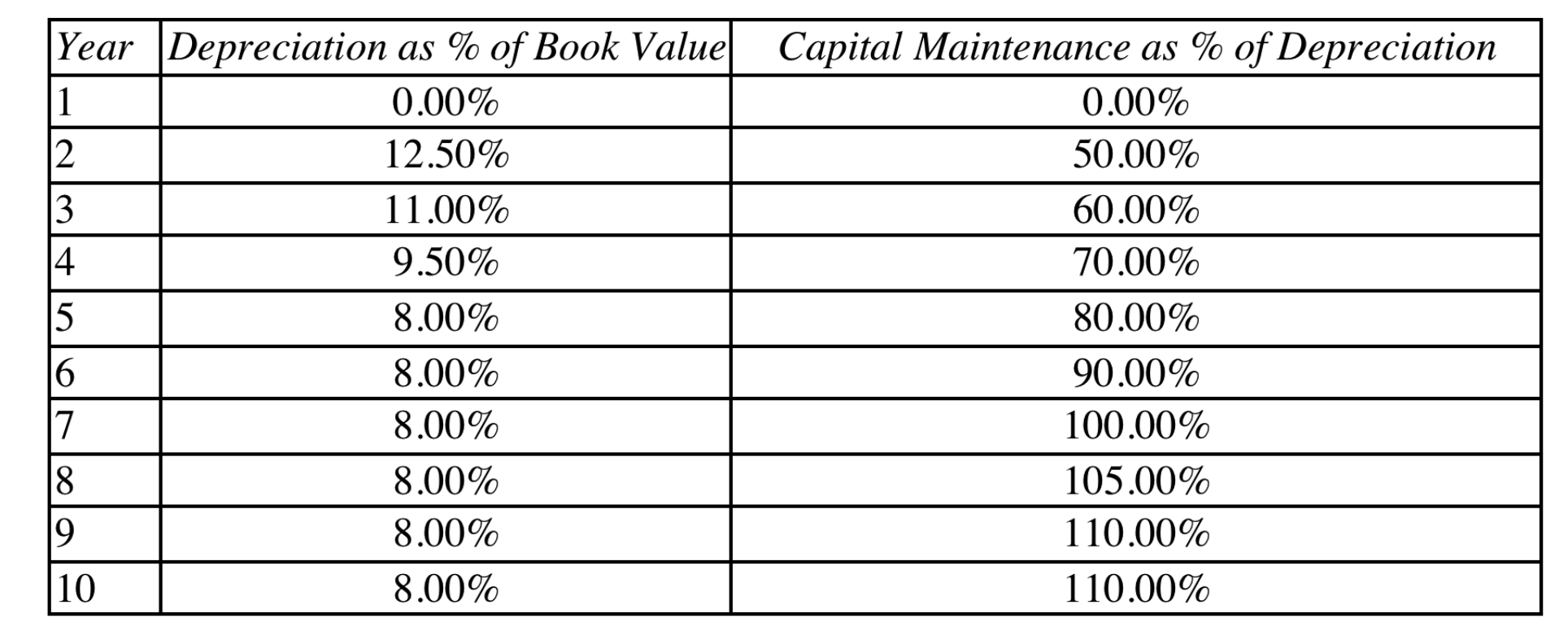
• as the park is new the maintainece is relatively cheap, but as the park ages it begins to grow as parts need replacing, machines age, refurbishments etc.

Accounting view of return

• Used to make a judgement on whether the return is worth relative to the investment

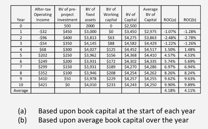
• take the after tax operating income that is estimated and scale it to the accounting investment

• Accounting investment is treating capex as part of book value and add on working capital invested each year to come out with a book capital at the start , end and average for each year, divide after tax income by this book value of capital

• This is the return on capital that is compared to the risk of the business unit

• This can also be compared with the cost of capital to determine the excess return the firm has made on its existing investments (to the extent u trust the numbers)

Estimating a hurdle rate for Disney’s Rio Project

• Therefore it is a bad investment right?

• However we only used 10 years, theme parks generally dont become cash cows in 10 years, see other theme parks, OG disney is 59 years old as of 2013, therefore we need to take a look at the bigger picture (Using TV)

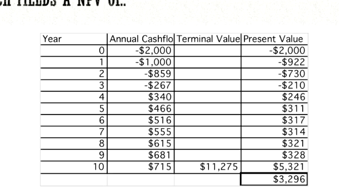
• This indicates the project should be accepted as the positive NPV suggests that disney will increase its value as a firm by $3296 Million

Risk premium for foreign objects

• The exchange rate should be diversifiable risk (hence should not command a premium) if:

  • the company has projects in many countries

  • the investors in the company are globally diversified

• the same diversification argument can be applied for some political risk which would mean that it too should not affect the discount rate

  • there are aspects of political risks especially in emerging markets that can be difficult to diversify ad may effect cash flows by reducing life or cash flows on the project

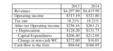
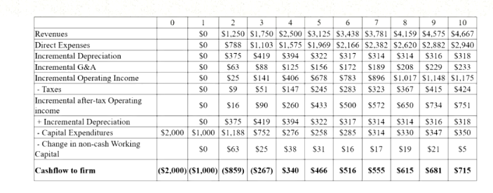
earnings to cash flow

• To get income from cash flow

  • add back all non cash changes such as depreciation, tax benefits:

  • subtract the CapEx

  • subtract the change in non-cash working capital

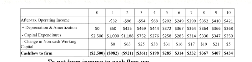
• First thing that is noticeable will be the CapEx spent on the first year,

Incremental cash flows

• Incremental costs are costs added by producingn one additional unit of a product or service

  • Easy way to think about is if nothing changes if i take or dont take this investment the item is not incremental

• Ensure that the cash flows are incremental as in are the cash flows acftually based on our decision to do the project

  • basically add back the sunk costs and G&A that is will be spent anyways

  • and subtract the tax depreciation tax benefit (next card)

• There is another way done by using incremental depreciation

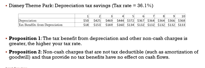
tax depreciation tax benefit

• although depreciation reduces taxable income and taxes, it is a non cash expense, the beenfit of depreication is therefore the tax benefit.

  • Tax Benefit = Depreciation * Tax Rate

• As we are depreciating the sunk costs the company would do that anyway therefore its not incremental

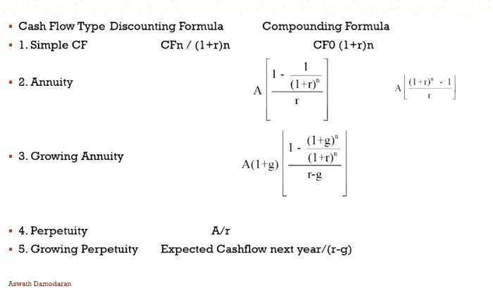
time weighted cash flows

• Incremental cash flows in the earlier years are worth more than incremental cash flows in later years

• Cash flows across time cannot be added up, they have to be brought to then same point in time before aggregation

• This process of moving cash flows is

  • discounting

  • compounding

DCF Measures of Return and decision rule

• Net Present Value (NPV): sum of present values of all cash flows from the project (including initial investments)

  • the cash flows must be discounted at the appropriate hurdle rate, COE or COC

  • Decision rule NPV > 0 accept

  • NPV is over and above the cost of capital therefore if NPV is $1 it’s $1 extra dollar we make

• Internal Rate of Return (IRR): discount rate that makes the net present value equal zero

  • percentage rate of return based upon incremental time-weighted cash flows

  • Decision rule: Accept if IRR > Hurdle Rate

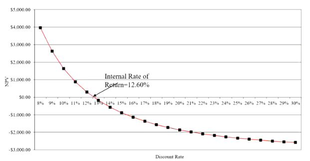
• The diagram above indicates that the project is a good one, given that the IRR is 12.60% higher than the cost of capital of 8.6% (NPV=0 when IRR is 12.6 where they cross the line essentially)

NPV vs IRR

• IRR and NPV will yield similar results most of the time; however, they can also yield different results as

  • A project can only have 1 NPV, whereas it can have more than 1 IRR

  • NPV is a dollar surplus value, while IRR is a percentage measure of return. NPV is larger for large-scale projects, while IRR is higher for smaller projects

  • NPV assumes that intermediate cash flows are reinvested at the hurdle rate which is based on what you can make on investments of comparable risk, while IRR assumes intermediate cash flows are reinvested at the IRR

    • might be a little dangerous to assume to use the IRR as if the IRR is really high we may not be able to meet the same return in future projects

Closure on Cash Flows (TV and SV)

• Salvage Value: In a project with a finite and short life, compute a salvage value which is the expected proceeds from selling all of the investment at the end of the project life. it is often equal to book value of fixed assets and working capital

• Terminal Value: In a project with an infinite or very long life, we compute cash flows for a reasonable period, and then compute a terminal value for this project which is the present value of all cash flows that occur after the estimation period ends

  • assuming project lasts forever, and that cash flows grow at the inflation rate forever, TV in Y10

    • CF in Year 11 / (Cost of Capital - Growth Rate) = 715 (1.02) / (.0846-.02) = $11275 Million

Project Analysis in different currencies

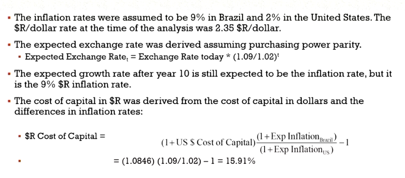
• Essentially by using the principle of PPP, we are able to predict the exchange rate of whatever currency we are using

• Formula (in this scenario)

Exchange rate of BRL/USD * (Expected inflation Brazil / Expected inflation US)

• Inflation is higher in Brazil than it is in the US, therefore it is expected that the BRL will depreciate (seen below)

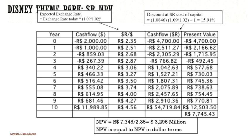
• However we also have to take into account the cost of capital (which is currently in USD) to convert to BRL, this is done by (at least in this case):

1 + Cost of Capital (US) * (Expected inflation of Brazil / Expected inflation of US)

• Note that the NPV is equal to NPV in dollar terms once we compute it using the BRL cost of capital,

Dealing with uncertainty

• Assuming forecasts are correct and one trusts the forecast, simply compute the cash flows until the time we get our money back that is invested into the project

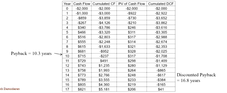
• many companies use payback constraints limiting the investments that payback in certain number of years (6/10 Years)

Simulating NPVs (Monte Carlo Simulation)

• used to analyse uncertainties, for example the likelihood of a scenario that the project only returns 20% of expected revenue to the firm (applied to revenue, risk premiums and other variables)

• in a monte carlo simulation there will be certain distrivtuons associated with different variables

• Also be aware of double-counting as a buffer may be added to the country risk premium for example

• Datapoints can come from historical data (past projects), peer comparisons or other subjective methods

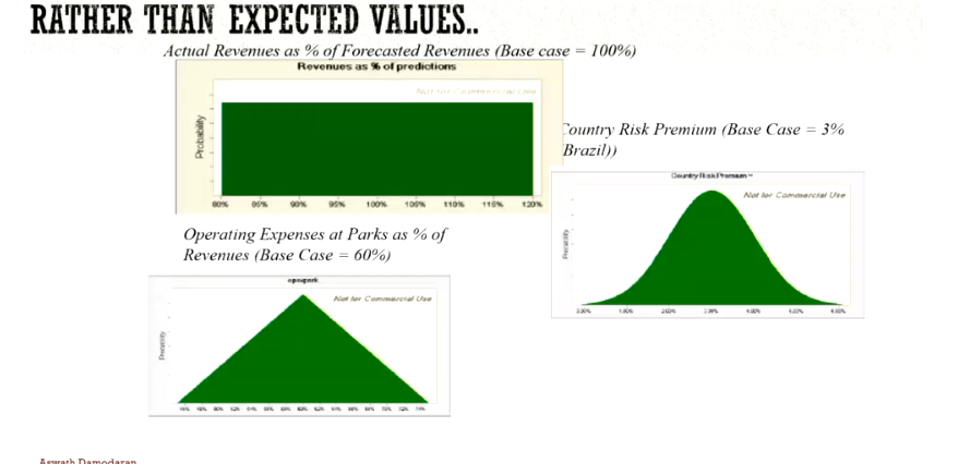
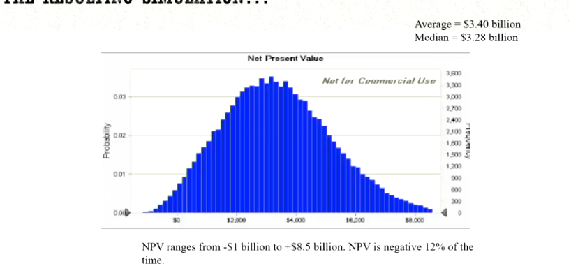
• Essentially take a drawing from each of these distributions (revenue, expenses, risk premium), generate a simulated NPV and repeat across a large number of times (10000, 1000, etc)

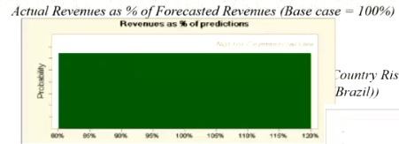
Uniform Distribution

• Essentially all outcomes are uniformly distributed, this means that there is equal chance of those outcomes occurring

Normal distribution

• There is just two parameters

  • mean

  • standard deviation

Triangular distribution

CHATGPT explain

Investment Project Abroad Assumptions Using Vale

See Damadoran

Effect of exchange rates on IRR and NPVs

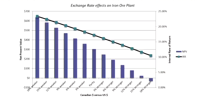
• The costs were largely in CAD for the project, therefore as the CAD appreciated against the USD, the NPV decreases

Hedging Diagram

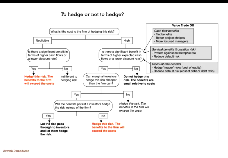
• Marginal investors can be very diversfied therefore they are not concerned with the currency risk

Acquisitions and Projects

• Acquisitions are projects / investments and should be treated as such by:

  • Having positive NPV, the present value of expected cash flows from the acquisition should exceed the price paid on the acquisition

  • The IRR of the cash flows to the firm (equity) from the acquisition > cost of capital (equity) on the acquisition

• In estimating the cash flows on the acquisition, count in any possible cash flows from synergies

• The discount rate to assess present value should be based on the risk of the investment (target company) and not the entity considering the investment (acquiring company)

Estimating cost of capital for an acquisition (Tata and Harman)

• This assumes that there are no synergies with the acquisition

Estimating the target company’s cash flows

• Operating Income

  • Find operating income for the most recent year + add back non-recurring expenses and adjust income for conversion of operating lease commitments to debt

  • Also remember the tax rate as it will be used for the effective tax rate for the cash flows

• Reinvestment

  • Find the most recent figures for depreciation, capital expenditures and acquisitions, and non cash working capital

• Also recall the growth rate of the firm which will be added to the estimates for variables like depreciation, CapEx, and operating income