Quantifying Species Diversity

What is the most important factor regulating populations?

• Food availability

• Abiotic factors

• Competition

• Facilitation

• Predation

• Herbivory

• Parasitism

Species diversity

depends upon richness and evenness

bottom-up control

population sizes and dynamic are regulated by the primary producer of the food web

evidence for bottom-up control

1. Energy decreases from plants through herbivores to carnivores

2. Organisms prefer food that contains the highest nitrogen content (NLH)

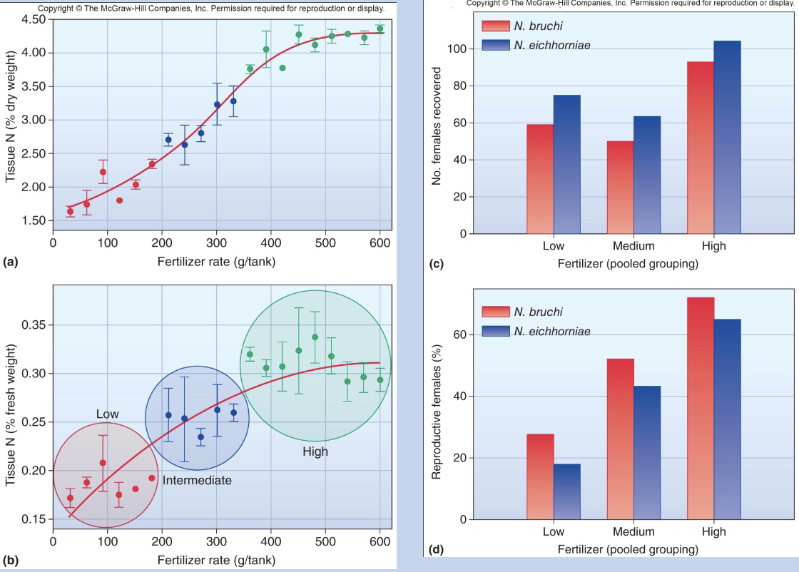
Example of bottom-up control(draw graph)

Bottom-up control of water hyacinth and its herbivores in Florida

trophic cascade(Top-down control)

highest level of food chain controls species size and dynamics

Evidence for Top-down control

1. Suggest that natural enemies control herbivores directly

2. Herbivores control plants directly – So natural enemies influence plants indirectly

3. Effects may percolate from predators through herbivores to plants

Examples of top-down control

• Biocontrol: Natural enemies such as predators and parasites are released against pests.

• Cottony Cushion Scale, California citrus and ladybird beetle

Necessary attributes for biocontrol agents

(Huffaker and Kennett, 1969)

1. General adaptability to the environment.

(Mismatch between enemy’s preferred optimal abiotic range and the released range: most common reason for failure (34.5%))

2. High searching capacity for hosts.

3. High rate of increase relative to the host’s.

4. Good dispersal ability.

5. Minimal time lag effects in responding to changes in host numbers

Twelve Guidelines for the International Code of Best Practices for Classical Biocontrol

1. Ensure the target weed”s potential impact justifies the risk of releasing nonendemic agents

2. Obtain multi-agency approval for the target weed

3. Select agents with the potential to control the target weed

4. Release safe and approved agent

5. Ensure only the intended agent is released

6. Use appropriate protocols for release and documentation

7. monitor impact on the target plant species

8. Stop releases of ineffective agents, or when control is achieved

9. Monitor impacts on potential nontarget species

10. Encourage assessment of changes in plant and animal communities

11. Monitor interactions among agents

12. Communicate the results to the public

Biological control often backfires

1. invasive species ladybeetle introduced for pest control takes over native ladybeetles habitat

2. Cane toad: to control grey backed beetle, but beetles at top of cane toads at the bottom, beetles during the day toads during the night, → toads spread everywhere, breed all year, poisonous and resistant to predator venom

Community

group of species that coexist and interact within a defined area

Based on observable differences in their physical and biological structure

– Can be difficult to define boundaries!

Ways to measure Diversity within communities

There are various kinds of diversity, and various ways to measure and compare diversity:

– Species richness

– Relative abundance

– Evenness and dominance

– Functional types or guilds

– Diversity of higher taxa (families, etc.)

– Genetic diversity within species

Species richness

the count of the number of species occurring within the community

Relative abundance

the percentage each species contributes to the total number of individuals of all species

Berger – Parker Index

the most simple dominance index

D_BP = N_max / N

1. N_max = total number of individuals in the most common species

2. N = the total number of individuals in the community

If one species tends to dominate, the community won’t be very diverse (and the index will be high)

To express greater diversity with a greater value, use the complement (D_BPC) = 1 - DBP

Simpson’s Index (D_S)

Probability of any two individuals drawn at random from a community belong to different species

• Where p_i is the proportion of individuals in the ith species (n_i/N)

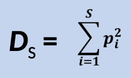
total dominance

When the basic Simpson index = 1, this represents total dominance (the converse of diversity)

Gini-Simpson Index

A complement index to Simpson’s [D_GS = (1 – D_S)]

– Increasing values mean increasing diversity

Simpson’s downsides

Heavily weighted towards the most abundant species

– Addition of rare species will rarely change the index.

– Limited value in conservation biology (but at least uses information about more species than Berger-Parker)

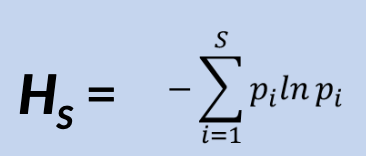
Shannon (or Shannon-Weiner) Index

Relative abundance of each species = pi = ni / N

• In the absence of diversity, where only one species is present, H_S = 0

• H_max = ln S, occurs when all species are present in equal numbers

Values for real communities often fall between 1.5 and 3.5, with the higher the value, the greater the diversity.

This index is very valuable to conservation biologists, who often study rare species and their importance to the community

Tells you certainty of guessing next species: PPPP_ is easier than LMTS_

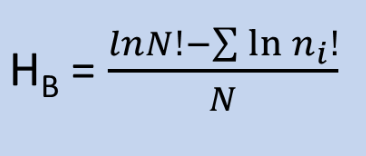
Brillouin Index

Where n¡ : number of individuals in each species and N is the total number of individuals of all species in the community

N! is a factorial

rare species with single individuals contribute nothing to the overall value of the index (ln1 = 0)

Shannon vs. Brillouin

The Brillouin index may have some advantage over the Shannon index related to conservation biology.

• Changes as overall abundance changes

The Shannon index is simple to use and doesn’t use factorials in the equations that produce huge numbers

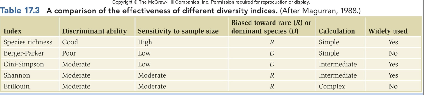
Which index to use?

Dominance

the degree to which a species is far more abundant (in numbers or biomass) than other species in a community

Evenness

how many individuals belong to each species—are they distributed fairly equally

For any information statistic index, maximum diversity is found when all species are equally abundant.

Evenness, E, compares the actual diversity to the maximum possible

For example, using the Shannon index:

E = H_S/H_max, H_max = ln S

E is constrained between 0 and 1.0 and can be determined using any of the indices

Diversity indices

A measure of the number of species in an area and the relative distribution of individuals among these species

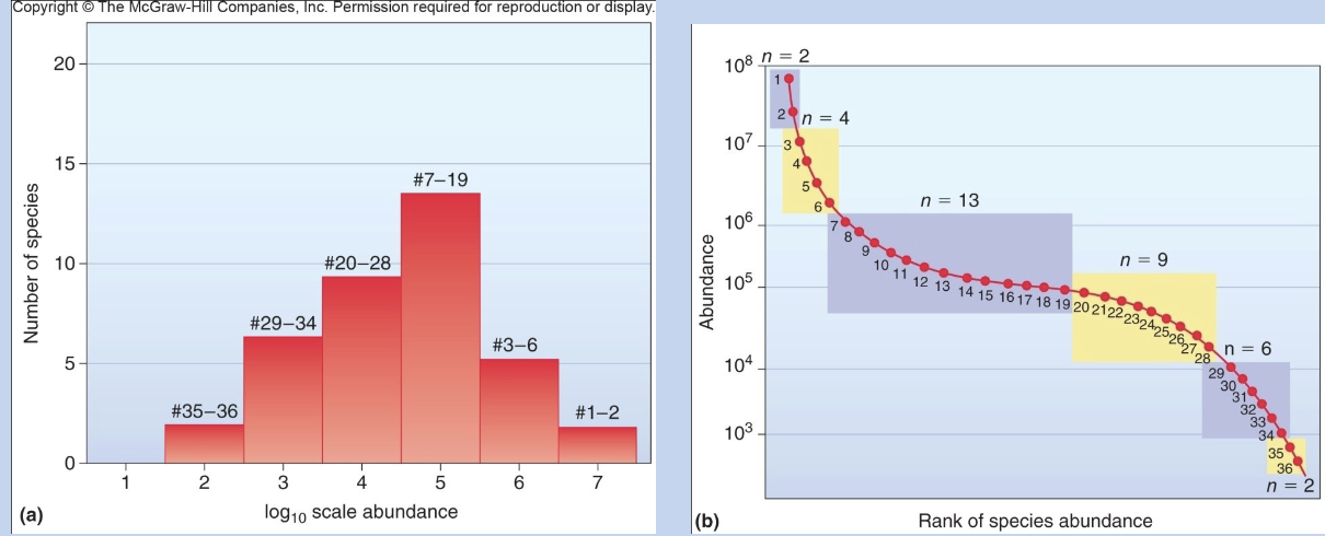
Rank abundance diagrams

Graphical plots of numbers of individuals/species against rank of species commonness in the community

making Rank Abundance diagrams

Plot the relative abundance(p_i) of each species against rank

– Ranks species by abundance (species w/ most individuals = rank 1)

– A community with a greater species evenness would have a more gradual slope of the rank-abundance curve

Plotting abundance (log scale) against rank gives a more complete picture of species in a community

Can be drawn for number of individuals, biomass of individuals, ground area covered by plants, etc

Rank abundance diagrams forms

– Lognormal

– The dominance preemption model

– The random fraction model

– The MacArthur fraction model

Log Normal Rank Abundance Plot

Similarity indices

Compare how areas may be similar in biodiversity, in terms of the numbers of species they hold in common

Community Similarity

Distinguishing between communities based on differences in species composition is important to understanding the processes that control community structure

Similarity indices types

Jaccard index

Sorensen’s index

Jaccard index

C_J = a/(a + b + c)

a = found in both sites

b = found in community B but not community A

c = found in community A but not community B

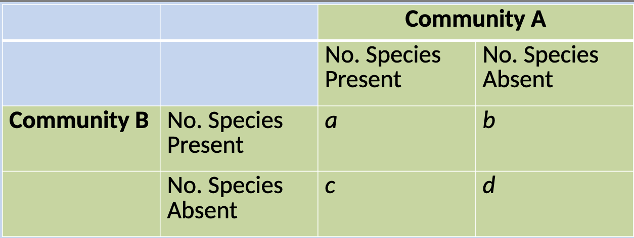
Sorenson index

C_S = 2a/(2a + b + c)

Weights matches in composition between sites more than mismatches due to the possibility of undersampling

How many species are there

Current counts (1.5 million +)

Estimated 8.7 million species

Species richness is underestimated

Assessing species richness depends on

– Number of samples

– Type of habitat

– Issues associated with taxonomy

It is not possible to sample everywhere

– Species accumulation curve

Quantifying biodiversity

Conduct surveys in a subset of sample areas (plots)

As you sample more subsets, more likely to accumulate more species

– Species accumulation curve rises rapidly at first, as more common species are quickly accumulated

– Rises more slowly as more rare species are included

– In principle, curve will asymptote when no new species are added despite increased sampling

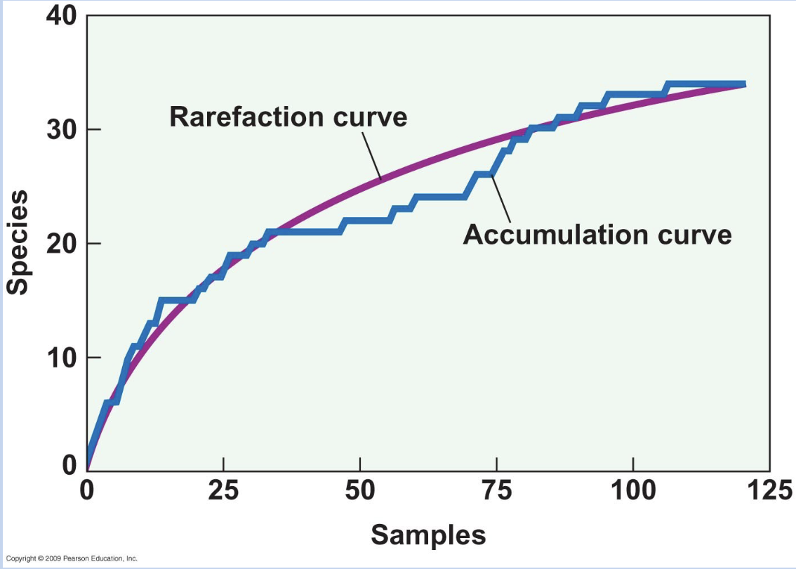
Survey graph

Asymptote = optimal sampling size and best estimate for number of species present

Accumulation curve: move left → right, species found(check this?)

Rarefaction curve: a graphical tool that plots the expected number of species against the number of individuals sampled

Estimating richness

When a species accumulation curve does not reach an asymptote, there are various methods that can be used to approximate where the curve is likely to plateau

Just because a species is present, it may not be detected within a survey!

In any given survey, a species may be:

– present (and detected)

– truly absent

– present (and undetected)

Additional methods to quantify biodiversity include this detection parameter

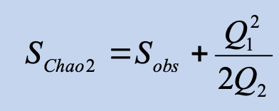
Chao 2 estimator

Where Q1 = number of species observed in only one sample, Q2 = number of species observed in only two samples

Why preserve biodiversity?

Benefits to humans

– Food, forest products, medicines

– Genetic resources

– Tourism and Aesthetic components

– Indirect (ecosystem services)

Investigating Species Richness Patterns

biodiversity is not distributed randomly

Latitudinal Species Gradient

number of species increases (in general) from polar → tropical

Hypotheses for diversity patterns

Difficult because…

– No one explanation explains all the patterns

– Different factors may act at different scales

– Patterns vary by taxonomic group

Area

There is more area at the equator – geometric fact

Species - Area hypothesis

Increased richness with increased area?

– More individuals (larger populations), resistance to extinction

– Greater range of habitats

– More potential for barriers that lead to speciation

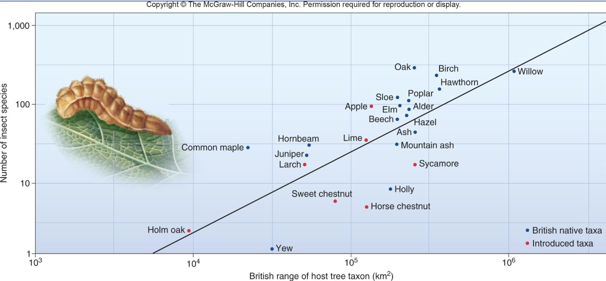
Species – Area hypothesis example

Relationship between insect species richness on British trees and area

Trees with a greater range support more insect species

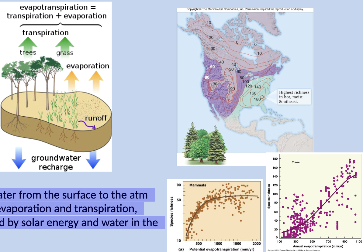
Species-Energy hypothesis

Environmental conditions favorable for photosynthesis and plant growth may give rise to increased plant diversity over evolutionary time

Provides a wider resource base permitting more species to coexist

– More herbivores, more predators, parasites, scavengers!

– Also provides habitat and structural diversity

Energy measured using evapotranspiration(imagine pictures)

Flux of water from the surface to the atm through evaporation and transpiration,

Influenced by solar energy and water in the ground

Species – energy doesn’t explain why

Some tropical areas have low productivity but high species richness

Some areas have high productivity but low species richness

– The sub-Antarctic Ocean

– Polluted waterways

– Estuaries

Favorability/Seasonality hypothesis

In a stable climate, species can specialize on predictable resources and have narrower niches

– Facilitating speciation

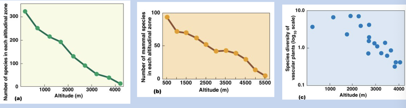
Fewer species have evolved to tolerate harsh or unfavorable environments (high latitudes, altitudes)

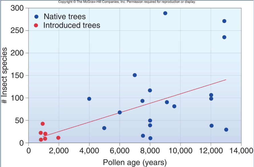
Species – Time Hypothesis

Tropics have been more stable across geologic time allowing more time for the evolution of new species

Temperate regions are younger than tropical regions and are still recovering from the Pleistocene glaciations

Species accumulation due to: Longer time for species in tropical areas

Alternatively, evolution is faster in the tropics

– High temperatures, short generation times, increased mutation rates

Support for Species-Time Hypothesis

number of insects in british trees by radiocarbon dating pollen

Older tree species support more insect species

Species-Time does not explain…

Data that do not support the hypothesis

– Ex: The oldest vertebrate lineages do not support more helminth parasites than the youngest lineages

Limited applicability to marine systems and endotherms

Data that suggest higher speciation and extinction rates in high latitudes

Null models: Mid-Domain

Mid-domain or boundary constraint models assume that hard boundaries constrain the size and placement of species’ ranges which causes randomly distributed species’ ranges to cluster near the center of the domain

Hypotheses for the latitudinal gradient

Why are there more species the farther you go from the poles?

a) area

b) energy

c) ambient energy/seasonality

d) time/historical stability

e) null models

Factors that promote local species richness

• Small change in environmental conditions

• Physically diverse habitat

• Evolution

• Middle stages of succession (more next time)

• Natural Enemies

• Intermediate environmental disturbance

Natural Enemies

Natural enemies reduce prey density, decrease prey competition, and permit coexistence of more prey species

Natural Enemies example

starfish(keystone species as well)

Intermediate Disturbance

maximum diversity at intermediate levels of disturbance

mix of r & K-selected species

High Rates of Disturbance

Species continually driven extinct

• Only good colonists (r-selected species) persist, moving in from adjoining, but undisturbed habitats

Low Rates of Disturbance

Competitively dominants outcompete all other species

A few K-selected species would persist, yielding low species richness

Intermediate Disturbance example

boulders at sea

Support for intermediate disturbance hypothesis

Higher tree diversity found in Japanese forests with intermediate storm intervals

(Hiura 1995).

• Coral reefs and tropical forests maintain high diversity in areas disturbed by hurricanes and tropical storms

Factors that negatively influence biodiversity

• Extreme conditions

• Large disturbance

• Intense environmental stress

• Severe shortage of key resources

• Isolation

• Introduction of invasive species

Invasive species pathway

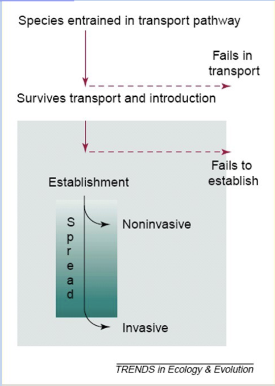
How do invasive species succeed?

Escape constraints of predators or parasites

Find vacant niches

Human disturbance aids their success

Have attributes that facilitate their success

Proposed attributes of successfully invading species

1. shedding of natural enemies during colonization

2. absence of natural enemies in recipient community

3. Better competitor than native species

4. Presence of mutualists in recipient community

5. high dispersal ability

6. association with humans

7. high reproductive rate (r-selected)

8. high growth rate (r-selected)

9. ability to thrive in disturbed areas

10. asexual reproduction (plants)

11. unique ways of lire; occupy vacant niches

12. climatic match between site of origin and site of colonization

Consequences of Plant Invaders

Can take over entire ecosystems

– Colorado saltcedar

– Passionflower in Hawaii

– European cheatgrass

Plant Invaders examples

– Colorado saltcedar

– Passionflower in Hawaii

– European cheatgrass

– Kudzu

Kudzu

Rapidly growing vine native to Japan, introduced in 1880’s as an ornamental and a forage crop

1900’s: Farmers encouraged to plant to resist erosion

Can grow as high as 30 meters tall

Thrives in ample sun

Quickly outcompetes native vegetation, strangling other plants and having the power to uproot tree

Plant Invaders - Aquatic

53 exotic aquatic weeds in Hudson River

– Alter animal species

– Choke waterways

– Change nutrient cycles

– Disrupt recreational activities

Vertebrate Invasions

Mammals

– Several escaped or were released into the wild

– Prey on native animals, plants, intensify erosion, vectors of disease

Birds

– Pigeon was intentionally introduced, now causes ~1.1 billion damages/year

Fish

– 138 introduced to US

– Can lead to extinction of natives

– Sport fishing 38 billion business

Effects of Invasions

Community composition

– Lead to homogenization

Negative impacts on native animals

Reducing the recruitment of natives (succession)

Promoting the spread of other non-native species

Ecosystem-level consequences

Methods of Control

Eradication is rare

Control depends on commitment and continued diligence

Long term, ecosystem-level efforts are the most successful

Prevention is the best way

What threatens species?

Habitat Degradation…..………………85%

Invasive Species……..………………..49%

Pollution………………………..……... 24%

Overexploitation……………..……….. 17%

Disease………………………..………. 3%

What is rarity?

Species that are at high risk are typically rare

Numerical: Factors associated with the abundance of a species

Spatial: Factors associated with the distribution of a species

Which species are most threatened?

Species differ in their susceptibility

– Life history characteristics

– Small metapopulations

– Seasonal migrators

– Specialized habitat requirements

– Large home range

– Species hunted/collected by humans

– Distribution

• Ubiquitous vs. Endemic

Identifying threatened species

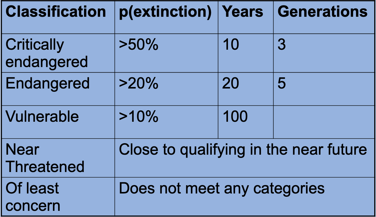
IUCN red list

Can incorporate spatial extent, population size, demography, stochastic events, but can be classified based on minimal data

Goals of IUCN red list

– Provide global index on the state of biodiversity degeneration

– Identify priority species for conservation attention

Classifying Extinction Risk table

Population approach to conservation

Endangered species consist of a few – or even a single local population(s)

– Often restricted to protected areas

Conservation plan requires the preservation of as many individuals as possible within the greatest possible area!

– …but space is limited…

How much space does this species need?

Determine MVP

Based on the MVP, determine area of suitable habitat needed (Minimum Dynamic Area)

Minimum Viable Population(MVP)

– Number of individuals needed to ensure that a species will persist in a viable state

– Depends on life history and dispersal ability

Protecting and Preserving: The Ecosystem Approach

Protect populations of species in their native habitats

– Preserve sufficient habitat areas through govt or privatization

– Eliminate or reduce populations of nonnatives

– Manage protected areas and restore natives

– Restore habitats

Protected Areas

An area of land and/or sea especially dedicated to the protection and maintenance of biological diversity, and of natural and associated cultural resources, and managed through legal or other effective means. (IUCN)

Is the PA system representative?

• Though Mexico has a lot of conservation reserves, only 33% of the amphibians occur in at least one protected area (Young et al 2004)

• In the eastern slope of the Andes, the endemic plants, amphibians, mammals and birds all have different distributions (Young et al 2007)

• Of the 11,633 species of mammals, amphibians, turtles, freshwater tortoises, and threatened birds analyzed, 12.2% (1424) of species are not covered by any protected area in the global network (Rodrigues et al. 2004a, b)

How do you choose an area to protect?

Reserve selection algorithms: selecting by maximizing the number of species in a reserve

– Typically based on presence/absence data, ignoring spatial heterogeneity and metapopulation dynamics (Akçakaya and Sjögren-Gulve 2000)

• Community-based approaches require an understanding of the relationship between biodiversity and the landscape

Hot Spots (Conservation International)

Patterns of species richness (and endemism!) increases as move from poles to equator

How can we support the most species for the least cost?

Mittermeier et al. (2004) identified 24 hotspots that contain 150,000 endemic plants (2.3% ELS)

Myers identified 25 hotspots that contain 133,149 plant species (44% known plants)

Where to place focus?

1. Biodiversity hotspots

2. Megadiversity countries (17 home to 80% species!)

3. Crisis ecoregions

– Areas at greatest risk of habitat loss because of land conversion

4. “Last of the wild”

– Areas that fall within the lowest 10% of human affected areas

– Pristine areas offer a great opportunity for conservationists because of their relatively intact communities

nine global biodiversity conservation priority templates

CE, crisis ecoregions

BH, biodiversity hotspots

EBA, endemic bird areas

CPD, centers of plant diversity

MC, megadiversity countries

G200, global 200 ecoregions

HBWA, high-biodiversity wilderness areas

FF, frontier forests

LW, last of the wild

make up the Priority setting exercises

What are the limitations of Global Priority Setting Exercises?

Difficulties in measuring taxonomic richness

Congruence between indicator groups (e.g. plants) and other elements of biodiversity?

Many rare species found in ‘cold spots’- sites of relatively low biological diversity

Source-sink dynamics complicate identification of hotspots

How will patterns change with climate change?